I think I was around 12 when I read about the famous thought experiment by Galileo that disproved the old notion of Aristotle that heavier bodies fall faster than lighter ones.

Suppose we have two stones, the first being lighter than the second. Release the two stones from a height to fall to Earth. Stone 2, being heavier than stone 1, falls more rapidly. If they are joined together, argues Galileo, then the combined object should fall at a speed somewhere between that of the light stone and that of the heavy stone since the light stone by falling more slowly will retard the speed of the heavier. But if we think of the two stones tied together as a single object, then Aristotle says it falls more rapidly than the heavy stone. How do the stones know if they are one object or two?

(Source)

I remember being stunned by the simplicity and elegance of the argument. No tower of Pisa needed, no pendulum, no inclined plane, nothing! Just a clever way of arranging thoughts.

In any case, I was telling my dad about this argument a couple of weeks ago. He asked me why then do pieces of paper fall to ground more slowly than rocks. It took me a few minutes to come up with a satisfactory answer.

Two questions then for you dear readers.

1. Where exactly does Galileo’s reasoning break down in the presence of air resistance?

2. What are your favorite examples of arguments in theoretical CS or math which are too clever for their own good?

This is the second of a two-part series on quantifier elimination over the reals. In the first part, we introduced the Tarski-Seidenberg quantifier elimination theorem. The goal of this post is to give a direct and completely elementary proof of this result.

Before embarking on the proof journey, there’s something we can immediately note. It’s enough to prove quantifier elimination for formulas of the following type:

$latex \displaystyle \phi(y_1,\dots,y_m) = \exists x \bigwedge_{i=1}^n \left( p_i(x,y_1,y_2,\dots, y_m)~\Sigma_i~ 0\right)&fg=000000$

where each $latex {\Sigma_i \in \{<,=,>\}}&fg=000000$ and each $latex {p_i \in {\mathbb R}[x][y_1, \dots, y_m]}&fg=000000$ is a polynomial over the reals. Why? Well, if one quantifier can be eliminated, then we can inductively eliminate all of them. And we can always convert the single quantifier to an $latex {\exists}&fg=000000$ by negation if necessary and then distribute the $latex {\exists}&fg=000000$ over disjunctions to arrive at a boolean combination of formulas of the type above.

I will try to describe now how we could “rediscover” a quantifier elimination procedure due to Albert Muchnik. My description is based on a very nice exposition by Michaux and Ozturk but with some shortcuts and a more staged revealing of the full details. The specific algorithm for quantifier elimination we describe will be much less efficient than the current state-of-the-art described in the previous post. The focus here is on clarity of presentation instead of performance.

We will complete the proof in three stages.

1. $latex {m = 0}&fg=000000$ and linear polynomials

First, let’s restrict ourselves to the simplest case: $latex {m = 0}&fg=000000$ and all the polynomials $latex {p_i}&fg=000000$ are of degree one. In fact, let’s even start with a specific example:

$latex \displaystyle \phi = \exists x ((x+1 > 0) \wedge (-2x+3>0) \wedge (x > 0))&fg=000000$

We will partition the real line into a constant number of intervals so that none of the functions changes sign inside any of the intervals. If we do this, then to decide $latex {\phi}&fg=000000$, we merely have to examine the finitely many intervals to see if on any of them, the three functions ($latex {x+1, -2x+3}&fg=000000$, and $latex {x}&fg=000000$) are all positive.

Each of the linear functions has one root and is always negative on one side of the root and always positive on the other. We will keep ourselves from using the exact value of the root, even though finding it here is trivial, because this will help us in the general case. Whether the function is negative to the left or right side of the root depends on the sign of the leading coefficient. So, the first function $latex {x+1}&fg=000000$ has a root at $latex {\gamma_1}&fg=000000$, is always negative to the left of $latex {\gamma_1}&fg=000000$ and always positive to the left.

The second function, $latex {-2x+3}&fg=000000$, has another root $latex {\gamma_2}&fg=000000$, is always negative to its right, and always positive to its left. How do we know if $latex {\gamma_2}&fg=000000$ is to the left or right of $latex {\gamma_1}&fg=000000$? Well, $latex {-2x+3 = -2(x+1) + 5}&fg=000000$, and since $latex {\gamma_1}&fg=000000$ is a root of $latex {x+1}&fg=000000$, it follows that $latex {-2\gamma_1 + 3 = 5 > 0}&fg=000000$. So, $latex {\gamma_1}&fg=000000$ is to the left of $latex {\gamma_2}&fg=000000$. This results in the following sign configuration diagram (for each pair of signs, the first indicates the sign of $latex {x+1}&fg=000000$, the second the sign of $latex {-2x+3}&fg=000000$):

Finally, the third function $latex {x}&fg=000000$ has a root $latex {\gamma_3}&fg=000000$, is always negative to the left, and always positive to the right. Also, $latex {x = (x+1)-1}&fg=000000$ and $latex {x=-\frac{1}{2}(-2x+3) + 1.5}&fg=000000$, and so $latex {x}&fg=000000$ is negative at $latex {\gamma_1}&fg=000000$ and positive at $latex {\gamma_2}&fg=000000$. This means the following sign configuration diagram:

Since there exists an interval $latex {(\gamma_3,\gamma_2)}&fg=000000$ on which the sign configuration is the desired $latex {(+,+,+)}&fg=000000$, it follows that $latex {\phi}&fg=000000$ evaluates to true. The algorithm we described via this example will obviously work for any $latex {\phi}&fg=000000$ with $latex {m=0}&fg=000000$ and linear inequalities.

2. $latex {m=0}&fg=000000$ and general polynomials

Now, let’s see what changes if some of the polynomials are of higher degree with $latex {m}&fg=000000$ still equal to $latex {0}&fg=000000$:

$latex \displaystyle \psi = \exists \left( \bigwedge_{i=1}^n p_i(x) \Sigma_i 0\right)&fg=000000$

where each $latex {\Sigma_i \in \{<,>,=\}}&fg=000000$. Again, we’ll try to find a sign configuration diagram and check at the end if any of the intervals is described by the wanted sign configuration.

If we try to implement this approach, a fundamental issue crops up. Suppose $latex {p_i}&fg=000000$ is a degree $latex {d}&fg=000000$ polynomial and we know that $latex {p_i(\gamma_1) > 0}&fg=000000$ and $latex {p_i(\gamma_2)>0}&fg=000000$. In the case $latex {p_i}&fg=000000$ was linear, we could safely conclude that $latex {p_i(x)}&fg=000000$ is positive everywhere in the interval $latex {(\gamma_1,\gamma_2)}&fg=000000$. Not so fast here! It could very well be for a higher degree polynomial $latex {p_i}&fg=000000$ that it becomes negative somewhere in between $latex {\gamma_1}&fg=000000$ and $latex {\gamma_2}&fg=000000$. But note that this would mean $latex {p_i’ = \frac{\partial}{\partial x} p_i}&fg=000000$ must change sign somewhere at $latex {\gamma_3 \in (\gamma_1, \gamma_2)}&fg=000000$ by Rolle’s theorem. New idea then! Let’s also partition according to the sign changes of $latex {p_i’}&fg=000000$, a degree $latex {(d-1)}&fg=000000$ polynomial. Suppose we have done so successfully by an inductive argument on the degree, and $latex {\gamma_3}&fg=000000$ is the only sign change occurring in $latex {(\gamma_1, \gamma_2)}&fg=000000$ for $latex {p_i’}&fg=000000$.

We now want to also know the sign of $latex {p_i(\gamma_3)}&fg=000000$. Imitating what we did for $latex {d=1}&fg=000000$, note that if $latex {q_i = (p_i \text{ mod } p_i’)}&fg=000000$, then $latex {p_i(\gamma_3) = q_i(\gamma_3)}&fg=000000$ since $latex {\gamma_3}&fg=000000$ is a root of $latex {p_i’}&fg=000000$. The polynomial $latex {q_i}&fg=000000$ is degree less than $latex {d-1}&fg=000000$, so let’s assume by induction that we know the sign pattern of $latex {q_i}&fg=000000$ as well. Thus, we have at hand the sign of $latex {p_i(\gamma_3)}&fg=000000$.

There are now two situations that can happen. First is if $latex {p_i(\gamma_3) > 0}&fg=000000$ or $latex {p_i(\gamma_3) = 0}&fg=000000$.

This is because $latex {p_i}&fg=000000$ reaches the minimum in $latex {(\gamma_1, \gamma_2)}&fg=000000$ at $latex {\gamma_3}&fg=000000$, and since $latex {p_i(\gamma_3) \geq 0}&fg=000000$, $latex {p_i}&fg=000000$ is not negative anywhere in $latex {(\gamma_1, \gamma_2)}&fg=000000$.

The other situation is the case $latex {p_i(\gamma_3)<0}&fg=000000$. By the intermediate value theorem, $latex {p_i}&fg=000000$ has a root $latex {\gamma_4}&fg=000000$ in $latex {(\gamma_1,\gamma_3)}&fg=000000$ and a root $latex {\gamma_5}&fg=000000$ in $latex {(\gamma_3, \gamma_2)}&fg=000000$.

Note again that because $latex {\gamma_3}&fg=000000$ is the only root of $latex {p_i’}&fg=000000$ in the interval $latex {(\gamma_1, \gamma_2)}&fg=000000$, there cannot be more than one sign change of $latex {p_i}&fg=000000$ between $latex {\gamma_1}&fg=000000$ and $latex {\gamma_3}&fg=000000$ and between $latex {\gamma_3}&fg=000000$ and $latex {\gamma_2}&fg=000000$.

So, from these considerations, it’s clear that knowing the signs of the derivatives of the functions $latex {p_i}&fg=000000$ and of the remainders with respect to these derivatives is very helpful. But of course, obtaining these signs might recursively entail working with the second derivatives and so forth. Thus, let’s define the following hierarchy of collections of polynomials:

$latex \displaystyle \mathcal{P}_0 = \{p_1, \dots, p_n\}&fg=000000$

$latex \displaystyle \mathcal{P}_1 = \mathcal{P}_0 \cup \{p’ : p \in \mathcal{P}_0\} \cup \{(p \text{ mod } q) : p,q \in \mathcal{P}_0, \deg(p)\geq \deg(q)\}&fg=000000$

$latex \displaystyle \dots&fg=000000$

$latex \displaystyle \mathcal{P}_{i} = \mathcal{P}_{i-1} \cup \{p’ : p \in \mathcal{P}_{i-1}\} \cup \{(p \text{ mod } q) : p,q \in \mathcal{P}_{i-1}, \deg(p)\geq \deg(q)\}&fg=000000$

$latex \displaystyle \dots&fg=000000$

The degree of the new polynomials added decreases at each stage. So, there is some $latex {k}&fg=000000$ such that $latex {\mathcal{P}_k}&fg=000000$ doesn’t grow anymore. Let $latex {\mathcal{P}_k = \{t_1, t_2, \dots, t_N\}}&fg=000000$ with $latex {\deg(t_1) \leq \deg(t_2) \leq \cdots \leq \deg(t_N)}&fg=000000$. Note that $latex {N}&fg=000000$ is bounded as a function of $latex {n}&fg=000000$ (though the bound is admittedly pretty poor).

Now, we construct the sign configuration diagram for the polynomials $latex {\{t_1, t_2, \dots, t_N\}}&fg=000000$, starting from that of $latex {t_1}&fg=000000$ (a constant), then adding $latex {t_2}&fg=000000$, and so on. When adding $latex {t_i}&fg=000000$, the real line has already been partitioned according to the roots of $latex {t_1, \dots, t_{i-1}}&fg=000000$. As described earlier, $latex {\text{sign}(t_i)}&fg=000000$ at a root $latex {\gamma}&fg=000000$ of $latex {t_j}&fg=000000$ is the sign of $latex {(t_i \text{ mod } t_j)}&fg=000000$ at $latex {\gamma}&fg=000000$, which has already been computed inductively. Then, we can proceed according to the earlier discussion by partitioning into two any interval where there’s a change in the sign of $latex {t_i}&fg=000000$. The only other technicality is that the sign of $latex {t_i}&fg=000000$ at $latex {-\infty}&fg=000000$ and its sign at $latex {+\infty}&fg=000000$ are not determined by the other polynomials. But these are easy to find given the parity of the degree of $latex {t_i}&fg=000000$ and the sign of its leading coefficient.

3. $latex {m>0}&fg=000000$ and general polynomials

Finally, consider the most general case, $latex {m>0}&fg=000000$ and arbitrary bounded degree polynomials. Let’s interpret $latex {{\mathbb R}[x,y_1,y_2,\dots, y_m]}&fg=000000$ as polynomials in $latex {x}&fg=000000$ with coefficients that are polynomials in $latex {y_1, \dots, y_m}&fg=000000$, and try to push through what we did above. We can start by extending the definitions of the hierarchy of collections of polynomials. Suppose $latex {p(x,\mathbf{y}) = p_D(\mathbf{y}) x^D + p_{D-1}(\mathbf{y}) x^{D-1} + \cdots + p_0(\mathbf{y})}&fg=000000$ and $latex {q(x,\mathbf{y}) = q_E(\mathbf{y}) x^E + q_{E-1}(\mathbf{y}) x^{E-1} + \cdots + q_0(\mathbf{y})}&fg=000000$ with $latex {d \leq D}&fg=000000$ the largest integer such that $latex {p_d(\mathbf{y}) \neq 0}&fg=000000$, $latex {e \leq E}&fg=000000$ the largest integer such that $latex {q_e(\mathbf{y}) \neq 0}&fg=000000$, and $latex {d \geq e}&fg=000000$. One problem is that $latex {(p \text{ mod } q)}&fg=000000$, as a polynomial in $latex {x}&fg=000000$, may not have polynomials in $latex {y}&fg=000000$ as its coefficients. To skirt this issue, let:

$latex \displaystyle (p\text{ zmod } q) = q_e(\mathbf{y}) p(x,\mathbf{y}) – p_d(\mathbf{y})x^{d-e} q(x,\mathbf{y})&fg=000000$

Then, whenever $latex {q(x,\mathbf{y}) = 0}&fg=000000$, the sign of $latex {p(x,\mathbf{y})}&fg=000000$ equals the sign of $latex {(p\text{ zmod } q)}&fg=000000$ at $latex {(x,\mathbf{y})}&fg=000000$ divided by the sign of $latex {q_e(\mathbf{y})}&fg=000000$. Moreover, $latex {(p \text{ zmod } q)}&fg=000000$ is a degree $latex {(d-1)}&fg=000000$ polynomial. So, we will want to replace mod by zmod when constructing the collections $latex {\mathcal{P}_i}&fg=000000$. All this is fine except that we have no idea what $latex {d}&fg=000000$ and $latex {e}&fg=000000$ are and what specifically the sign of $latex {q_e(\mathbf{y})}&fg=000000$ is. Recall that $latex {\mathbf{y}}&fg=000000$ is an unknown parameter! So, what to do? Well, the most naive thing: for each polynomial $latex {p}&fg=000000$, let’s just guess whether each coefficient of $latex {p}&fg=000000$ is positive, negative, or zero.

Now, we can define the hierarchy of collections of polynomials $latex {\mathcal{P}_0, \mathcal{P}_1, \dots}&fg=000000$ in the same way as in the previous section, except that here, the polynomials are in $latex {{\mathbb R}[x,y_1, \dots, y_m]}&fg=000000$, we use zmod instead of mod, and each time we add a polynomial, we make a guess about the signs of its coefficients. The degree of the newly added polynomials decreases at each stage, so that there’s some finite bound $latex {k}&fg=000000$ such that $latex {\mathcal{P}_k}&fg=000000$ doesn’t grow anymore. We can now run the procedure described in the previous section to find the sign configuration diagram for $latex {\mathcal{P}_k}&fg=000000$. In the course of this procedure, whenever we need to know the sign of the leading coefficient of a polynomial, we use the value already guessed for it. Finally, we check whether any interval in the sign configuration diagram contains the desired sign pattern.

Consider the whole set of guesses we’ve made in the course of arriving at this sign configuration diagram. Notice that the total number of guesses is finite, bounded as a function of $latex {n}&fg=000000$. Now, let’s call the set of guesses good if it results in a sign configuration diagram that indeed contains an interval with the wanted sign pattern. Our final quantifier-free formula is a disjunction over all good sets of guesses that checks whether the given input values of $latex {y_1, \dots, y_m}&fg=000000$ is consistent with a good set of guesses.

I attended the FSTTCS conference that was held in IIT Bombay last December. The conference saw over 180 participants and had many interesting talks. I will discuss a few of them in this post.

Talks from Breakthroughs in TCS workshop

Madhu Sudan. Multiplicity Codes: Locality with High Efficiency.

Madhu Sudan gave a nice talk based on a recent result by Swastik Kopparty, Shubhangi Saraf and Sergey Yekhanin (STOC 2011). He was excited about the result for two reasons. Firstly, unlike other advances in LDCs where applications of the results are found only in other parts of theory, this result actually could be of great practical interest. “It’s the numbers that are making sense” he said. Secondly, the construction of the code is so elegant that you are surprised by its simplicity.

I’ll try to sketch the main idea below:

Background. Suppose we want to send a k-bit message on a noisy channel. A well-known method is to use an error-correcting code to encode the k-bit message x into an n-bit codeword C(x) and transmit the codeword instead of the message x. The codeword C(x) is such that we can recover the original message x from it even if many bits in C(x) get corrupted. A typical way to recover x would be to run a decoder on the (possibly corrupted) C(x).

Two parameters in this scheme are of interest: the redundancy incurred in constructing the codeword C(x) and the efficiency with which we can decode the message x from the codeword. The complexity of encoding is usually ignored since it is not critical in most applications.

The rate of the code is the ratio of message length to codeword length: k/n. The higher the rate, the lesser the redundancy of the code.

LDCs. But what if one is interested only in knowing just a particular bit of the message x? This is where a Locally Decodable Code (LDC) is useful. LDCs allow the reconstruction of any arbitrary bit x_i by looking only at a small number of randomly chosen positions of the received codeword C(x). The query complexity of the code is the number of bits we need to look at in order to recover a particular bit.

Obviously, we desire to have LDCs with high rate and low query complexity. But until now, for codes with rate>1/2, it was unknown how to construct any non-trivial decoding. For rates lower than 1/2, we could construct a code with rate O(ε^Ω(1/ε)) and query complexity O( k^ε) for 0<ε<1. For example, Reed-Muller codes — which are based on evaluating multivariate polynomials.

Bivariate Reed-Muller codes. We briefly describe how polynomials can be useful in coding. Let F_q denote the finite field of cardinality q. Consider the bivariate polynomials over the field F_q. A bivariate polynomial of degree d has ( {d+1 \choose 2} ) monomials. For example, if d=2 the monomials are x²,xy and y². So any polynomial of degree d can be specified by the coefficients of each of these monomials. The coordinates of the message x can be thought of as coefficients of a polynomial P(x,y) of degree d. So our message is of length ( k={d+1 \choose 2} ). Each coordinate of the message has a value from F_q (we call this an alphabet). The codeword C(x) corresponding to the message x is obtained as follows: The coordinates of the codeword is indexed by elements of ( F_{q}^2 ). So the length of the codeword n=q².

The codeword corresponding to the polynomial P(x,y) is the vector C(P) as given below:

So the first co-ordinate of C(P) would have the value of P(1,1), the second coordinate would have the value of P(1,2), and in general the (i*q+j)th coordinate of C(P) would have the value P(i,j).

The rate of this code is less than 1/2 and it can be shown that the correct value at a particular coordinate of the received codeword can be decoded by making only O(√k) queries on the received codeword, assuming that a constant fraction of the codeword gets corrupted.

Multiplicity codes. The key idea in the paper is to encode the message using multivariate polynomials and their partial derivatives. If we plug this idea to the above example, each coordinate of the codeword will have 3 alphabets instead of one or in other words each coordinate would be a value from ( F_{q}^3 ). So the codeword is now:

This improves the rate from <1/2 to 2/3! It can be done without increasing the query complexity. This by itself is a new result. What’s more is they can extend this idea to get codes of arbitrarily high rate while keeping the query complexity small. Here is their main theorem from the paper:

For every ε>0, α>0, and for infinitely many k, there exists a code which encodes k-bit messages with rate 1-α, and is locally decodable from some constant fraction of errors using O(k^ε) time and queries.

Umesh Vazirani. Certifiable Quantum Dice.

Background. Many computational tasks such as cryptography, game theoretic protocols, physical simulations, etc. require a source of independent random bits. But constructing a truly random device is a hard task. Even assuming that such a device is available, how do we test if it is working correctly? This task seems impossible since a perfect random number generator must output every n bit sequence with equal probability and there is no reason one can reject a particular output in favor of an other.

Quantum mechanics offers a way to get past this fundamental barrier: starting with O(log² n) random bits one can generate n certifiable random bits.

To get an idea of how this is possible let us consider the CHSH game first (given below).

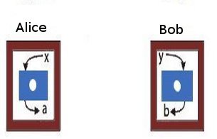
The CHSH game. Alice and Bob are two co-operating players who receive inputs x and y, respectively from a third party. Alice and Bob are at two different locations. The winning condition for them is to produce outputs a and b such that the following condition is satisfied: If x=y=1, then a and b must be different. For any of the other three combinations of x and y, the outputs have to be equal. If the players are correlated according to the laws of classical physics, only any three of the four pairs of inputs can be satisfied. So the maximum probability of winning is 0.75. However, if they adopt a strategy based on quantum correlations, this value can be increased to 0.851. See the references in this article in Nature for more details.

We can define a quantum regime corresponding to the success probabilities between 0.75 and 0.85. It is simple to construct two quantum devices corresponding to any value in the regime. But if two devices produce co-relations in the regime, they must be randomized. Or in other words, randomness is for real! This gives a simple statistical test to cerfify randomness.

Result. We are using two random input bits (x,y) to produce two random output bits, so this doesn’t accomplish much. We cannot claim the output to be more random than the input. Vazirani and Vidick in their paper describe a protocol that uses O(log ² n) seed bits to produce n certifiable random bits.

Jaikumar Radhakrishnan. Communication Complexity of Multi-Party Set-Disjointness Problem.

Consider the following problem: Alice and Bob are given inputs x and y respectively and are asked to compute a function f(x,y). They are charged for the number of bits exchanged. The minimum number of bits that have to be exchanged in order to compute the function f is the communication complexity of the problem. A particular problem that is of interest in the area of communication complexity is the set-disjointness problem.

Problem. There are k parties each of whom has a subset from {1,..,n} stuck on his forehead. Each party can see the all the subsets except his own. The set-disjointness problem is to determine if the intersection of all the k subsets is empty. Again, we charge for the number of bits exchanged. All the parties have access to a shared blackboard on which they can write, so we have a broadcast medium.

The case when k=2 is well-understood both in both deterministic and randomized settings. (In randomized version, all the parties have access to a shared source of infinite random bits.)

Results. Until recently, for the general multi-party case, the best lower bound on communication complexity known for the number-on-the-forehead model was Ω(n^1/k+1/2^{k^2}). Last year, Sherstov improved this bound to Ω(n/4^k)^1/4 which is close to tight.

Jaikumar is a fantastic teacher. In what was basically a blackboard-talk, he gave an overview of the main ideas in Sherstov’s proof in a way that was accessible even to non communication-complexity experts. The arguments are based on approximating Boolean functions by polynomials.

Other talks in BTCS

There were several other good talks. Naveen Garg surveyed the recent progress on approximation algorithms for the Traveling Salesman Problem that achieve a strictly better than 1.5 approximation factor. Manindra presented the result on lower bound on ACC by Ryan Williams. Aleksender Madry gave two talks: one in which he presented a new randomized algorithm for the k-server problem that achieves poly-logarithmic competitiveness and one on approximating max-flow in capacitated, undirected graphs using the techniques from electrical flows and laplacian systems. Nisheeth Vishnoi discussed new algorithms for the Unique Games Conjecture. Amit Kumar gave a talk about a recent result by Friedman, Hansen and Zwick on proving lower bounds for randomized pivoting rules in simplex algorithm. Sanjeev Khanna spoke about some recent progress on the approximability of the edge-disjoint paths problem. Most of these results are now famous in theory-circles.

Conference talks

There were 38 papers out of which about 16 were from Theory A. Here are some of the talks I attended:

The Semi-stochastic Ski-rental Problem. (Aleksander Mądry and Debmalya Panigrahi)

An online algorithm is an algorithm which optimizes a given function when the entire input in not known in advance, but is rather revealed sequentially. The algorithm has to make irrevocable choices about the output as the input is seen. The ratio of the performance of the online algorithm to the optimal offline algorithm is called the competitive ratio of the algorithm.

On one hand, we have online models which assume nothing about the input and on the other we have stochastic models which assume that the input comes from a known distribution. The semi-stochastic model in this paper unifies these two extremes. In this model, the algorithm does not know the input distribution initially, but can learn the distribution by asking queries. The algorithm has a certain query budget. If the budget is zero (resp. infinite), the model reduces to the online (resp. stochastic) version. The goal is to maximize the competitive ratio assuming that the queries are answered adversarially.

This model is well-motivated because in many real world situations, the online model is too pessimistic and the stochastic model is too optimistic. We can usually learn the input distribution to some extent and often learning the distribution incurs some cost.

Problem. The ski-rental problem is studied in this framework. The problem is as follows: Ann wants to go skiing, but she does not know the exact number of days she would like to ski. Each morning she has to decide if she has to rent a pair of skis or buy them. Renting the skis cost 1 unit/day and buying them would cost b units. The goal is to minimize the total cost.

Here is a trivial 2-competitive algorithm: Rent the skis for b-1 days. If she decides to go on the bth day, then buy them. This is the best one can do in a deterministic setting. The best randomized algorithm gives a competitive ratio of e/(e-1).

Results. Given a desired competitive ratio e/(e-1)+ε, the paper gives lower and upper bounds on the number of queries that need to be asked in order to achieve that ratio. The lower bound is C/ε (where C is a universal constant) and the upper bound is O(1/ε^1.5).

Rainbow Connectivity: Hardness and Tractability. Prabhanjan Ananth, Meghana Nasre, and Kanthi K Sarpatwar.

Problem. In an edge-colored graph, a rainbow path is a path in which all the edges have different colors. Given a graph G, can we color the edges using k colors such that every pair of vertices has a rainbow path between them? In short, is rc(G) ≤ k? A graph is said to be rainbow connected if the above condition is satisfied. Further, for every pair, if one of the shortest paths between them is a rainbow path, then the graph is said to be strongly rainbow connected (src(G)).

Results.The paper shows that determining if src(G) ≤ k is NP-hard even for bipartite graphs. The hardness of determining if rc(G) ≤ k was open for the case when k is odd. The authors establish the hardness for this case (for every odd k≥3) by an indirect reduction from vertex coloring problem. The argument is combinatorial in nature. I’m not sure if the same argument can be tweaked for the case when k is even (which might simplify the overall proof of hardness for every k≥3.)

Simultaneously Satisfying Linear Equations Over F₂. (by Robert Crowston et. al)

Problem. We are given a set of m equations containing n variables x₁,…,x_n of the form ∏_i∈Ix_i=b. The x_is and b take values from {-1,1}. For example, equations can be x₁x₄x₈=1, x₂x₅x_n=-1, etc. Each equation is associated with a positive weight. The objective is to find an assignment of variables such that the total weight of the satisfied equations is maximized.

The problem is known to be NP-Hard, so we concentrate on a special case. Let the total weight of all the equations be W. If we randomly assign 1 or -1 to each variable, every equation gets satisfied with probability 1/2. Hence, there is always an assignment that is guaranteed to give a weight of W/2. The problem MAX-LIN[k] is to find the complexity of finding an assignment with weight W/2+k, where k is the parameter.

Roughly, a problem is said to be fixed-parameter-tractable (FPT) is if an input instance containing n input bits and an integer k (called the parameter) can be solved in time f(k)n^O(1), where f(k) depends only on the parameter k.

Results. The authors show that the problem MAX-LIN[k] is FPT and admits a kernel of size O(k² log k) and give an O(2^{O(klog k)}(nm)^c) algorithm. They also have new results for a variant of the problem where the number of variables in the equation is fixed to a constant. The results in the paper is built on the previous results by the same authors some parts of which use Fourier analysis of pseudo-Boolean functions. I’m not familiar with these techniques.

Obtaining a Bipartite Graph by Contracting Few Edges. (by Pinar Heggernes et. al)

Problem. Given a graph G, can we obtain a bipartite graph by contracting k edges? This problem though simple to state was not studied before. Which is quite surprising considering that the related problem of removing vertices to obtain a bipartite graph is a central problem in parametrized complexity.

Results. The main result of the paper shows that the problem is fixed-parameter-tractable when parametrized by k. The result makes use of many techniques well-known in parametrized complexity like iterative compression, irrelevant vertex and important separators. An interesting open question is to decide if the problem admits a polynomial kernel.

The update complexity of selection and related problems. (Manoj Gupta, Yogish Sabharwal, and Sandeep Sen)

Problem. We want to compute the function f(x₁,x₂,…,x_n) when the x_is are not known precisely but rather just known to lie in an interval. We are allowed to query and update a particular variable, to get a more refined estimate. Each query has some cost. The objective is to compute the function f with minimum number of queries.

Results. The previous literature focuses on the case when the query returns the exact value of the variable. This paper generalizes the model by allowing query updates that return open or closed intervals or points instead of exact values. The performance of the online algorithm is compared against an offline algorithm that knows the input sequence and therefore is able to ask the minimum number of queries to an adversary. For some selection problems and MST, the authors show that a 2-update competitive ratio holds for the general model.

Optimal Packed String Matching. (by Oren Ben-Kiki et. al)

Problem. Given a text containing n characters find if a string of m characters appears in the text.

Results. This is an age-old problem. The paper considers the packed string matching case where each machine word can hold up to α characters. The paper presents a new algorithm that extends the Crochemore-Perrin constant-space O(n) algorithm to run get an O(n/α) algorithm. Thus achieving a speed-up of factor α. The packed string matching problem is also-well studied. What is different in this paper is that they achieve better running times by assuming two instructions that have become recently available on processors: one is string-matching instruction WSSM which can find a word of size α in a string of size 2α and the other is WSLM instruction which can find the lexicographically maximal-suffix in a word.

Physical limits of communication. (Invited talk by Madhu Sudan)

Given a piece of copper wire, what is stopping us from transmitting infinite number of bits in unit time on it? The is a fundamental question in communication theory. There could be two reasons why the capacity could be unbounded. Firstly, the signal strength is a real value so there are infinite number of them. Secondly, there are infinitely many instances of time at which a signal can be sent. The first possibility is ruled out due to the presence of noise. It appears that the delay in transmission time rules out the second possibility too, but this has not been extensively studied.

This paper studies this problem in a model where the communicating parties can divide the time into any number of slots but have to cope up with (possibly macroscopic) delays. The surprising result is that the capacity of the channel is bounded only when either noise or delay is adversarially chosen. If both the error sources are stochastic (or if noise is adversarial but independent of stochastic delay) then the capacity of the channel is infinite!

There were other invited talks by Susanne Albers, Moshe Vardi, John Mitchell, Phokion Kolaitis and Umesh Vazirani. Unfortunately, I missed many of these talks.

On the lighter side

TCS Crossword

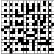
Try these:

• A confluence of researchers that generates fizz? (4)
• Fundamental fight (6,4)
• If the marking is right, it will fire! (8)

Find more clues like these and the grid in the TCS Crossword that was handed out to attendees during a coffee-break.

Algorithmic Contest (for students)

There was an algorithmic-contest as part of the conference (hosted on Algo Muse). Here is a take-away puzzle:

Contiguous t-sum problem. Given an array A[1..n] and a number t as input, find out if there exists a sub-array whose sum is t. For example, if the input is the array shown below and t=8, the answer is YES since A contains the sub-array A[2..4] whose sum is t. Prove an Ω(n log n) lower bound for the above problem on a comparison model.

Editors’ foreword

The current post, our first of 2012, is different from others we have published on this blog, and we have created a new category for it: Opinion.  In brief, the author, Guillaume Aupy, opposes the controversial US bill SOPA, and encourages readers to boycott Elsevier for its support of the passage of SOPA.

Rather than state an additional opinion about this topic — which would be out of place in an editor’s foreword anyway — we would like to note that, for better or for worse, internet censorship in an attempt to control copyright infringement is gaining traction in many countries, not just the USA. Most dramatically, just a few days ago, a court in Finland ordered a major internet service provider there to block access to The Pirate Bay — and the web page of the organization that brought the lawsuit fell under a Distributed Denial of Service attack from Anonymous Finland, which has threatened long term action if the Supreme Court doesn’t reverse the IP block.  Even more recently, a Dutch court ordered a block on The Pirate Bay on 11 Jan 2012.  Spain is scheduled to enact a “SOPA-like” law before March 2012.  However, there are already at least three new mirror sites for The Pirate Bay that are (currently) unaffected by any court order, and, of course, it is possible for Finns to visit the blocked sites using an anonymous browsing tool such as The TOR Network.

Given the international context, the US opposition to SOPA is relatively strong.  The popular web site Reddit plans a twelve-hour blackout to protest SOPA on January 18th, GoDaddy withdrew its support of SOPA after losing tens of thousands of customers from a boycott, and there is even a Boycott SOPA smartphone app that scans an item’s barcode and tells the user whether the company that made the item is on the list of supporters for SOPA.  Aupy’s request in the post below is that theoretical computer scientists engage in a similar action.

Main post: Boycott Elsevier for supporting SOPA

The Stop Online Piracy Act (SOPA) is a bill that would allow the U.S. Department of Justice, as well as copyright holders, to seek court orders against websites accused of enabling or facilitating copyright infringement (Wikipedia). My intention here is not to rewrite in a worst fashion what other people already wrote about SOPA, but if you have never heard of this bill before, I really urge you to go read the Wikipedia article, so you can see by yourself in how many ways this bill is wrong. If it can convince you to read about SOPA (and make up your mind), know that opponents of the bill include Google, Facebook, Twitter, the Wikimedia Foundation (these organizations even “talked” about a blackout as SOPA protest (see here and here)), but also eBay, Mozilla Corporation, and human rights organizations such as Reporters Without Borders, the Electronic Frontier Foundation, the ACLU, and Human Rights Watch.

 

There are however supporters of the SOPA bill. Amongst the many supporter is Elsevier, which I imagine many of you know as a publisher of a lot of TCS journals. It is time for us, the scientific community to raise our voice. A good way may be to

1. Refusing to serve as peer reviewers to Elsevier journals.
2. Not submitting papers to Elsevier journals.
3. If you are an Editor-in-Chief or in the editorial board, let the right people hear about your opinion.

 

And if this is not enough an argument to boycott Elsevier,  you may also want to remember the 2009 scandal where Elsevier published fake journals as covert advertisements for pharmaceutical companies.

On 7/11/2011, I asked the question with the same name on the parent site. More precisely:

How important is knowing how to code in TCS (in fields where programming is not directly involved) : is there reasons which could bring a Computational Complexity theorist (for example) to know how to code? Is it worth spending a lot of time learning how to code? And if there are, is there a category (functional, imperative, object-oriented..) of programming language that would be more suited? I can imagine that someday I may have to implement some algorithms for my work, but then can I wait for this moment? Or is there something more?

I got so many good answers that I was advised to blog about it. This is my ‘grand debut’ so forgive me for my prose. I will not give every answers, only the part which I though were the most helpful to me. The rest of the answers can be found on the original question.

Reasons

1. Testing a Conjecture by Tsuyoshi Ito

Testing a conjecture with numerical calculation can save the time which would have been spent in vain trying to prove a false statement.

1.5 Visualization by John Moeller

A computer is a great tool, it allows you for instance to see in different dimensions that are hard to imagine. Being able to see stuff helps for new ideas.

2. Theoretical results are not always real results by Suresh Venkat

Some optimal algorithms could be really hard to implement, and then not usable in practice, maybe an algorithm not as efficient but that can be implemented would be a better result. It opens up new theoretical research direction.

3. Type-Checking your proofs by Alessandro Cosentino

Learning a functional language forces you to type-check your programs, which can be a big asset for later when you start to type-check your proofs. This statement was however shaded by Sasho Nikolov who stated that even though this was true, maybe it was not worth the time if this was the only reason to learn a functional language.

4. Teaching by Martin Berger

There is a chance that someday a researcher in a university will be given courses with a substantial programming component. Being already comfortable can help being a better teacher.

5. If you know you will need to learn someday, the sooner the better by Peter Shor

Otherwise when you will really need it you will not have time for it.

6. Programming can be fun by Tsuyoshi Ito

Comment +1’d by 11 people! That says it all I guess.

Languages

1. (Strongly-Typed) Functional

(+) Teach to type-check, useful for proofs.

(+) A must for the logic/PL semantics field.

(-) Time consuming

(-) Hard to “see” things (see argument for imperative language).

2. Object-Oriented

(+) easy to learn and implement simple algorithms

(+) A must for software engineers (modular re-usable code)

(-) If you do not want to re-use it, not necessary to go that far (see Imperative)

3. Imperative

(+) Get a feel of what’s fast and what’s slow

(+) A must for people interested in efficient algorithms and data structures

(+) Widely used, almost “everyone” has a C compiler (if you want people to use your implementation).

To conclude, I got a lot of interesting answers, answers I did not think of before, so i am really grateful. If you have more arguments pros or cons (there was not that many argument against learning to program when you do not directly need it), feel free to add them. I will probably learn to program in C thanks to this useful discussion (in case some wondered what my final decision was :)). I think it took over my phlegm.

Oh, and also, I learned that “Euclid was a very crappy programmer”.

This post is by David Pritchard and Lev Reyzin.

Last Friday (11/11) was Theory Day at Georgia Tech. In fact, it was also Theory Day in NYC, although nobody seems to think the choice of date was coordinated or the start of a new national holiday. In Atlanta, Georgia Tech invited Avi Wigderson to give two talks on Thursday (making for two theory days in a row!), one for the broader public and then a math-on-whiteboard talk in the afternoon; and on Friday, there were four talks: by Thomas Dueholm Hansen, Mohit Singh, Alexander Mądry, and Ryan Williams, all aimed at theoreticians.

Dave: I was pretty impressed by the quality of the talks, which were about an hour long, and therefore gave the speakers quite a good chance to get into a bit of the technical details that are usually skipped at conferences. I have skimmed a couple of the papers before and really got much more intuition with these in-person explanations. Avi’s second talk was probably the most self-contained, on aspects of coding and a generalized Erdős/Gallai/Melchior/Sylvester theorem.  Also, we found that Alex may be a pyromaniac, since his examples for the k-server problem involved houses burning down (which you could think of as data requests). I was also pretty impressed by the quality of the lunch, which was a buffet of Indian food.

Lev: While I was a graduate student at Yale and during my year at Yahoo! Research in New York, I attended all the New York Theory Days for 5 years straight, so I was glad to see catch on in Atlanta too.  Apparently, we have Zvi Galil (now Georgia Tech’s College of Computing dean) to thank for the ideas of starting both the New York and the Atlanta theory days — so while the dates were not coordinated, the Theory Days, in some sense, were.  All four talks were great.  I especially enjoyed Alexander Mądry’s great and accessible talk on his recent progress on the k-server conjecture.  Ryan Williams also gave a very nice talk on how algorithms for circuits can imply lower bounds; it gave me some intuitive understanding that I didn’t have before.  Finally, I should note that I seem to remember the talks being filmed, so I’m hoping the videos will show on on Georgia Tech’s ARC website sometime.

If any readers attended the NYC Theory Day, please share your impressions in the comments!

I attended the 62nd Midwest Theory Day last Sunday, November 13rd. Usually there are two such theory days each year, but this was the only one in 2011. The event is like an informal workshop: anyone who wishes may sign up to speak, there are also invited speakers, lunch is provided, and there is no proceedings. Nicole Immorlica organized the event, and did a great job: there was a full day of talks, the room was great, the food was as good as any conference I’ve been to, and the invited speakers were entertaining and educational. 

Yael Tauman Kalai gave the first invited talk.  She gave a high-level overview of some hot topics in cryptography.  For example, she provided intuition into results she and co-authors obtained about designing systems whose algorithms resist physical attacks on cryptosystems.  A dramatic physical attack is someone who wants to break into a SIM card, so cooks it in a microwave oven for a while; this can cause bits to flip in the secret key, and even modify the circuitry of the SIM card itself.  (Some other examples of physical attacks are here.) Tauman Kalai presented a formalism in which the attacker could determine the system’s secret key, but would still be unable to produce a second secret key matching the system’s public key, unless the attacker used exponential resources or broke a reasonable cryptographic assumption.  For a system that can defend itself against an adversary capable of obtaining continual memory leakage of the system, see the FOCS 2010 paper Cryptography Resistant to Continual Memory Leakage (co-authors Brakerski, Katz, Vaikuntanathan).

Adam Kalai was the other invited speaker; he provided an overview of his ITCS 2011 paper Compression Without a Common Prior: an Information-Theoretica Justification for Ambiguity in Natural Language (co-authors Juba, Khanna, Sudan).  His talk was controversial: quite a few members of the audience either didn’t get his point, or got it and didn’t agree.  The idea, as I understand it, is to produce a mechanism two computers can use to compress and decompress messages they send to each other, even if their respective compression dictionaries (or “priors”) are different.  The motivation is how natural language works: you and I don’t have the same definitions for all words (and very different life experience) and yet we can communicate pretty well most of the time (for purposes of the example anyway).  If the message is large enough, one could of course use an algorithm like Lempel-Ziv, which approches best-possible compression in the limit.  But perhaps we just want to send one image, instead of thousands, and we would like to take advantage of the fact that both computers have useful priors for what an image is, even if those priors are not the same.  The paper provides an information-theoretic framework for this, but there is, as yet, no implementable algorithm.

There was also a day full of 15- and 20-minute talks by students, postdocs and faculty.  I will completely arbitrarily limit myself to the talks of the two people who sat on either side of me at lunch.  Fortunately, I thought both their talks were great.

Paolo Codenotti presented some brand new work on the group isomorphism problem: Polynomial-Time Isomorphism Test for Groups with no Abelian Normal Subgroups (co-authors Babai, Qiao).  This work extends the SODA 2011 paper Code Equivalence and Group Isomorphism (co-authors Babai, Grochow, Qiao).  The problem solved is the following: let $latex G$ be a group on $latex n$ elements, given to us as its multiplication table of size $latex n^2$.  Let $latex H$ be another group on $latex n$ elements, given in the same way.  If we know that $latex G$ and $latex H$ contain no normal subgroups that are abelian (i.e., commutative), then we can determine whether $latex G$ and $latex H$ are isomorphic in polynomial time.  One example of such a group is $latex A_5$, the alternating group on 5 elements, which has order $latex n=60$.  Another example would be any group built from direct sums of copies of $latex A_5$.

Tyson Williams gave an overview of his ITCS 2011 paper, Gadgets and Anti-Gadgets Leading to a Complexity Dichotomy (co-authors Cai, Kowalczyk).  Williams has also posted his slides from this talk online.  This paper is in the general category of holographic algorithms, a remarkable subfield of counting complexity started by Les Valiant and explored by Jin-Yai Cai, Williams’s advisor.  Since the slides are online, and the intuition behind the paper’s approach is so visual, I will let the slides speak for themselves, and close this post by simply stating the paper’s main theorem.

Theorem. Over 3-regular graphs $latex G$, the counting problem for any binary, complex-weighted function $latex f$,  $latex \displaystyle Z(G) = \sum_{\sigma:V \rightarrow \{0,1\}} \prod_{(u,v) \in E} f(\sigma(u),\sigma(v))$ is either polynomial-time computable or #P hard.  Furthermore, the complexity is efficiently decidable.

 The formalism of $latex f$ captures a wide variety of problems on 3-regular graphs, such as #VertexCover (how many vertex covers are there for the input graph), which is #P hard.

by Arnab Bhattacharyya

 

About a month ago, Ankur Moitra dropped by my office. We started chatting about what each of us was up to. He told me a story about a machine learning problem that he was working on with Sanjeev Arora, Rong Ge, and Ravi Kannan. On its face, it was not even clear that the problem (non-negative rank) was decidable, let alone solvable in polynomial time. But on the other hand, they observed that previous work had already shown the existence of an algorithm using quantifier elimination. Ankur was a little taken aback by the claim, by the power of quantifier elimination. He knew of the theory somewhere in the back of his mind, in the same way that you probably know of Brownian motion or universal algebra (possible future topics in this “Something you should know about” series!), but he’d never had the occasion to really use it till then. On the train ride back home, he realized that quantifier elimination not only showed decidability of the problem but could also be helpful in devising a more efficient algorithm.

Quantifier elimination has a bit of a magical feel to it. After the conversation with Ankur, I spent some time revisiting the area, and this post is a consequence of that. I’ll mainly focus on the theory over the reals. It’s a remarkable result that you definitely should know about!

1. What is Quantifier Elimination?

A zeroth-order logic deals with declarative propositions that evaluate to either true or false. It is defined by a set of symbols, a set of logical operators, some inference rules and some axioms. A first-order logic adds functions, relations and quantifiers to the mix. Some examples of sentences in a first-order logic:

$latex \displaystyle \forall x~ \exists y~(y = x^2)&fg=000000$

$latex \displaystyle \forall y~ \exists x~(y = x^2)&fg=000000$

$latex \displaystyle \forall x,y~((x+y)^2 > 4xy \wedge x-y>0)&fg=000000$

The above are examples of sentences, meaning that they contain no free variables (i.e., variables that are not bounded by the quantifiers), whereas a formula $latex {\phi(x_1,\dots,x_n)}&fg=000000$ has $latex {x_1, \dots, x_n}&fg=000000$ as free variables. A quantifier-free formula is one in which no variable in the formula is quantified. Thus, note that a quantifier-free sentence is simply a proposition.

Definition 1 A first-order logic is said to admit quantifier elimination if for any formula $latex {\phi(x_1,\dots,x_n)}&fg=000000$, there exists a quantifier-free formula $latex {\psi(x_1,\dots,x_n)}&fg=000000$ which is logically equivalent to $latex {\phi(x_1,\dots,x_n)}&fg=000000$.

If the quantifier elimination process can be described algorithmically, then decidability of sentences in the logic reduces to decidability of quantifier-free sentences which is often a much easier question. (Note though that algorithmic quantifier elimination of formulas is a stronger condition than decidability of sentences.)

2. Quantifier Elimination over the Reals

The real numbers, being an infinite system, cannot be exactly axiomatized using first-order logic because of the Löwenheim-Skolem Theorem. But the axioms of ordered fields along with the intermediate value theorem yields a natural first-order logic, called the real closed field. The real closed field has the same first-order properties as the reals.

Tarski (1951) showed that the real closed field admits quantifier elimination. As a consequence, one has the following (Seidenberg was responsible for popularizing Tarski’s result):

Theorem 2 (Tarski-Seidenberg) Suppose a formula $latex {\phi(y_1,\dots,y_m)}&fg=000000$ over the real closed field is of the following form: \begin{equation*} Q_1x_1~Q_2x_2~\cdots Q_nx_n~(\rho(y_1,\dots,y_m,x_1,\dots,x_n)) \end{equation*} where $latex {Q_i \in \{\exists,\forall\}}&fg=000000$ and $latex {\rho}&fg=000000$ is a boolean combination of equalities and inequalities of the form:

$latex \displaystyle f_i(y_1,\dots,y_m,x_1,\dots,x_n) = 0&fg=000000$

$latex \displaystyle g_i(y_1,\dots,y_m,x_1,\dots,x_n) > 0&fg=000000$

where each $latex {f_i}&fg=000000$ and $latex {g_i}&fg=000000$ is a polynomial with coefficients in $latex {{\mathbb R}}&fg=000000$, mapping $latex {{\mathbb R}^{m+n}}&fg=000000$ to $latex {{\mathbb R}}&fg=000000$. Then, one can explicitly construct a logically equivalent formula $latex {\phi'(y_1, \dots, y_m)}&fg=000000$ of the same form but quantifier-free. Moreover, there is a proof of the equivalence that uses only the axioms of ordered fields and the intermediate value theorem for polynomials.

I should be more explicit about what “explicitly construct” means. Usually, it is assumed that the coefficients of the polynomials $latex {f_i}&fg=000000$ and $latex {g_i}&fg=000000$ are integers, so that there is a bound on the complexity of the quantifier elimination algorithm in terms of the size of the largest coefficient. (If the coefficients are integers, all the computations only involve integers.) But, even when the coefficients are real numbers, there is a bound on the “arithmetic complexity” of the algorithm, meaning the number of arithmetic operations $latex {+, -, \times, \div}&fg=000000$ performed with infinite precision.

A quick example. Suppose we are given an $latex {r}&fg=000000$-by-$latex {s}&fg=000000$ matrix $latex {M = (M_{i,j})}&fg=000000$, and we’d like to find out whether the rows of $latex {M}&fg=000000$ are linearly dependent, i.e. the following condition:

$latex \displaystyle \exists \lambda_1, \dots, \lambda_r \left( \neg \left(\bigwedge_{i=1}^r (\lambda_i = 0)\right) \wedge \bigwedge_{j=1}^s (\lambda_1 M_{1,j}+\lambda_2 M_{2,j} + \cdots \lambda_m M_{r,j} = 0) \right)&fg=000000$

Tarski-Seidenberg immediately asserts an algorithm to transform the above formula into one that does not involve the $latex {\lambda_i}&fg=000000$’s, only the entries of the matrix. Of course, for this particular example, we have an extremely efficient algorithm (Gaussian elimination) but quantifier elimination gives a much more generic explanation for the decidability of the problem.

2.1. Semialgebraic sets

If $latex {m=0}&fg=000000$ in Theorem 2, then Tarski-Seidenberg produces a proposition with no variables that can then be evaluated directly, such as in the linear dependency example. This shows that the feasibility of semialgebraic setsis a decidable problem. A semialgebraic set $latex {S}&fg=000000$ is a finite union of sets of the form:

$latex \displaystyle \{x \in {\mathbb R}^n~|~f_i(x) = 0, g_j(x) > 0 \text{ for all }i=1,\dots, \ell_1, j= 1,\dots, \ell_2\}&fg=000000$

where $latex {f_1,\dots, f_{\ell_1}, g_1,\dots, g_{\ell_2}: {\mathbb R}^n \rightarrow {\mathbb R}}&fg=000000$ are $latex {n}&fg=000000$-variate polynomials over the reals. The feasibility problem for a semialgebraic set $latex {S}&fg=000000$ is deciding if $latex {S}&fg=000000$ is empty or not. An algorithm to decide feasibility directly follows from applying quantifier elimination.

Note that this is in stark contrast to the first-order theory over the integers for which Godel’s Incompleteness Theorem shows undecidability. Also, over the rationals, Robinson proved undecidability (in her Ph.D. thesis advised by Tarski) by showing how to express any first-order sentence over the integers as a first-order sentence over the rationals. This latter step now has several different proofs. Poonen has written a nice survey of (un)decidability of first-order theories over various domains.

2.2. Efficiency

What about the complexity of quantifier elimination over the reals? The algorithm proposed by Tarski does not even show complexity that is elementary recursive! The situation was much improved by Collins (1975) who gave a doubly-exponential algorithm using a technique called “cylindrical algebraic decomposition”. More precisely, the running time of the algorithm is $latex {poly(C,(\ell d)^{2^{O(n)}})}&fg=000000$, where $latex {C}&fg=000000$ measures the size of the largest coefficient in the polynomials, $latex {\ell}&fg=000000$ is the number of polynomials, $latex {d}&fg=000000$ is the maximum degree of the polynomials, and $latex {n}&fg=000000$ is the total number of variables.

A more detailed understanding of the complexity of quantifier elimination emerged from an important work of Ben-Or, Kozen and Reif (1986). Their main contribution was an ingenious polynomial time algorithm to test the consistency of univariate polynomial constraints: given a set of univariate polynomials $latex {{f_i}}&fg=000000$ and a system of constraints of the form $latex {f_i(x) \leq 0}&fg=000000$, $latex {f_i(x) = 0}&fg=000000$ or $latex {f_i(x) > 0}&fg=000000$, does the system have a solution $latex {x}&fg=000000$? Such an algorithm exists despite the fact that it’s not known how to efficiently find an $latex {x}&fg=000000$ that makes the signs of the polynomials attain a given configuration. Ben-Or, Kozen and Reif also claimed an extension of their method to multivariate polynomials, but this analysis was later found to be flawed.

Nevertheless, subsequent works have found clever ways to reduce to the univariate case. These more recent papers have shown that one can make the complexity of the quantification elimination algorithm be only singly exponential if the number of quantifier alternations (number of switches between $latex {\exists}&fg=000000$ and $latex {\forall}&fg=000000$) is bounded or if the model of computation is parallel. See Basu (1999) for the current record and for references to prior work.

As for lower bounds, Davenport and Heintz (1988) showed that doubly-exponential time is required for quantifier elimination, by explicitly constructing formulas for which the length of the quantifier-free expression blows up doubly-exponentially. Brown and Davenport (2007) showed that the doubly exponential dependence is necessary even when all the polynomials in the first order formula are linear and there is only one free variable. I do not know if a doubly exponential lower bound is known for the decision problem when there are no free variables.

---

Thanks to Ankur for helpful suggestions. Part II of this post will contain a relatively quick proof of Tarski’s theorem! Stay tuned.

 

Alfred Tarski (1951). A Decision Method for Elementary Algebra and Geometry Rand Corporation

Many CSTheory people probably know there is a new StackExchange Q&A site, Theoretical Physics, which is now in public beta, and was originally started by Joe Fitzsimons, co-editor of this blog.  My purpose for this post is to give TCS people a heads-up that there are now 16 questions on that site under the quantum-computing tag and the quantum-information tag that may be of interest to theoretical computer science.

My favorite of these questions is Rigorous Security Proof for Wiesner’s Quantum Money?  In this question, Scott Aaronson asks for an explicit upper bound on a value that is “known to exist” according to folklore, but that he and a co-author were unable to find in the literature or derive. Master’s student Abel Molina solves the problem, using a formalism of Gutoski and Watrous.  John Watrous then verifies the solution’s correctness.  There are also contributions by Dan Gottesman and Peter Shor.

In related news, there is now a proposal for a Quantum Information question and answer site on the Stack Exchange Area 51.  This proposal is (mildly) controversial, though, because some people are concerned it would duplicate topics already available on Theoretical Physics.

The 17th Conference on DNA Computing and Molecular Programming (DNA 17) was held Sept. 19-23 in Pasadena, California, at Caltech. In previous years the conference was held in early summer, but from now on it will be late summer/early fall in order to stagger 6 months apart from its sister conference FNANO (Foundations of Nanoscience), held every April in Snowbird, Utah.

The conference is not dedicated to theoretical computer science, of course, but like many inter-disciplinary fields such as algorithmic game theory or computational biology, theoretical computer science finds its way into many results in the field. As Luca Cardelli said during the conference, while the computing revolution was about the systematic manipulation of information, nanoscience is about the systematic manipulation of matter, so it is not surprising that theoretical computer scientists are finding interesting problems in this area.  I find it fascinating to watch a speaker prove a result relating DNA self-assembly to context-free grammars, just before the next speaker shows atomic force microscopy images of a self-assembled DNA nanostructure.

There’s always some impedance mismatch when experimentalists and theorists in any field get together to talk, but I believe our field promotes excellent cross-communication. The program committee, for instance, had members from the following university departments:

• Biological Chemistry and Molecular Pharmacology (1)
• Computer Science (17)
• Biophysics (1)
• Chemistry (4)
• Mathematics (1)
• Electrical Engineering (3)
• Bioengineering (3)
• Bioinformatics (4)
• Physics (2)
• Computation & Neural Systems (1)
• Cognitive Science (1)
• Systems Biology (1)

Interesting Conference Features

First I want to discuss some interesting features of the conference that I think could be beneficially adopted by general TCS conferences (some of these we are already seeing in TCS). As one of the local organizers, I was partially responsible for implementing some of these ideas, and I think it was worth the effort.

Tutorials

The first day was dedicated to three 90-minute lecture-style tutorials (slides available), and in parallel, there was an all-day wet-lab tutorial run by Elisa Franco, Josh Bishop, and Jongmin Kim,¹ in which the students constructed a chemical oscillator based on Jongmin’s and Elisa’s work on constructing chemical oscillators from DNA and transcription enzymes. Most of the tutorial attendees were theoreticians who wanted to see what all the fuss was about in the lab. It seems that about half of the oscillators worked properly on the first try. (They only got one try because the period of the oscillation is a few hours, so they had to run overnight.)

Tracks

One interesting aspect of the conference is the tracks, designed to appeal to both theoretical and experimental researchers. Track A looks familiar to TCS people: 15-page extended abstracts that appear in the conference’s LNCS proceedings. These are usually later submitted to CS journals such as SICOMP or TCS, or perhaps in the special issue of invited papers in Natural Computing associated with the DNA conference. Track B submissions are 1-page abstracts submitted for oral presentation only. Authors must provide a full paper for the program committee to judge, but the paper is not published. This is because Track B submissions are experimental results destined for eventual publication in physical science journals such as Nature, Science, or PNAS. These journals have much stricter requirements than CS journals regarding prior publication, so it is critical to the Track B presenters that nothing they submit can be construed as a publication.

Track C is posters, which are very common at physical science conferences and starting to make some headway at TCS conferences. I think posters are a great way to present your research, and I think the TCS community should adopt poster sessions at every conference. Maybe the person you most wanted to see your talk won’t attend it, but you can always grab them in the hallway and drag them over to your poster. It’s a great way to meet big shots in the field. There were three 90-minute poster sessions, with every poster at every session, and we encouraged the presenters to keep their posters up the whole week. This way, you could stand by your poster for a while, but you could also feel free to walk around to other posters without worrying that someone won’t get a chance to hear you explain your poster while you are away.

Panels

The panels consisted of four top researchers sitting at a table. Each gave a 5 minute talk about their vision for the future of the field, and then the audience could ask questions or heckle them for the next 25 minutes. These were a lot of fun. I think students especially benefited from the perspective given by high-level discussion of long-term research goals.

Impromptu Sessions

The impromptu sessions were a great idea, and I think all conferences could benefit from them. I think of them as a formalization of the idea that “the real conference interaction happens in the hallways” (as Lance Fortnow likes to remind us.) Often graduate students are intimidated by the idea of walking up to a couple of famous big-wigs talking in the hallway, even if they are talking about the student’s research area. For the impromptu sessions, there was a wiki where over the course of the week, anyone could schedule a session on any topic in a number of rooms that were reserved for the sessions. The sessions were required to be public, and I found it to be a great way for people to get together to chat about interesting problems, while inviting anyone else interested in the same problem to listen in or participate.

Theoretical Computer Science Results

I will highlight a few theoretical results that I found interesting. There were of course many great experimental results, and a lot of great CS talks on topics such as simulation, but since this is a TCS blog, I will focus on my favorite TCS-style results.

Self-Assembly and Context-Free Grammars

The winners of the best student paper award were Andrew Winslow and Sarah Eisenstat, for their excellent paper One-Dimensional Staged Self-Assembly, with Erik Demaine and Mashhood Ishaque.² Fix a finite alphabet $latex \Sigma$ and a finite set $latex G$ of “glues”. A tile type is a square labeled with a symbol from $latex \Sigma$, with its east and west sides labeled with (different) glues from $latex G$ (such tiles, both 1D and 2D, can be experimentally implemented with DNA). Initially all tile types start in separate test tubes. When two test tubes are mixed, any tile can bind to the west of any other tile if the first tile’s east glue matches the second tile’s west glue. Subsequent mixing may bind whole rows of tiles together. After each mixing, it is assumed that individual tiles are washed away so that only terminal assemblies (assemblies that cannot attach to anything else in the tube) remain.

The goal: design a fixed set of tile types so that any string over $latex \Sigma$ can be “spelled” by efficiently mixing the tiles in the correct order. How efficiently? The authors show that if each intermediate test tube is required to contain only one terminal assembly, then the number of mixing stages required to spell the string $latex x$ is within a constant multiplicative factor of the smallest context-free grammar that produces the singleton language $latex \{x\}$ (and they show that this bound is tight).

What does this mean? There is a linear-time $latex O(\log n)$-approximation algorithm for finding the smallest context-free grammar representing a string in this way (due to Sakamoto), which automatically translates to a linear-time algorithm for finding efficient mixing protocols for self-assembling one-dimensional patterns (implemented by the authors; here is an efficient mixing to spell the final verse of Edgar Allen Poe’s “The Raven” with DNA tiles).

However, if intermediate mixing stages are allowed to contain multiple terminal assemblies, even though the final stage is required to have only one terminal assembly (the assembly spelling $latex x$), then the number of mixing stages can be dramatically reduced (by a multiplicative factor of at least $latex \frac{n}{\log n}$).

Fuel-Efficient Computation with DNA Strand Displacement

My favorite paper was Less Haste, Less Waste: On Recycling and its Limits in Strand Displacement Systems, by Anne Condon, Alan Hu, Jan Manuch and Chris Thachuk. There has been a flurry of experimental and theoretical papers in the past few years based on a technique known as DNA strand displacement. It was shown by Soloveichik, Seelig, and Winfree that arbitrary chemical reactions can be “implemented” by DNA using the strand displacement reaction.³ Non-mass-conserving reactions such as $latex A \to A + B$ are implemented by extra “fuel” species assumed to be in abundance, so that the underlying implementation of $latex A \to A + B$ would consume fuel molecules and produce waste molecules, none of which corresponds to the abstract species $latex A$ or $latex B$.

Anne, Alan, Jan, and Chris showed how to implement a simple and pervasive computation — a counter that iterates through $latex 2^n$ different states using $latex O(n)$ different species — while consuming only $latex O(n^3)$ total fuel molecules (and producing the same amount of total waste molecules). A naïve implementation would consume fuel at every step, using $latex \Omega(2^n)$ fuel.

However, their counter requires that certain species have exactly one molecule present in solution, a tall order to implement experimentally. A more robust counter would work even with many copies of each species present, i.e., if many counters were thrown in together, they would each independently iterate from $latex 1$ to $latex 2^n$, without interfering with each other.

My favorite theorem in the paper shows this task to be impossible.4 In particular, they show a contrapositive result: any chemical reaction system (not just those implemented by DNA strand displacement) with $latex n$ species that is tolerant to having many copies of the system all reacting at once, has the property that any species is producible after $latex O(n^2)$ steps. In other words, if there is some species $latex S_{\text{end}}$ whose presence signifies the “end” of computation, there is no way to deterministically visit more than quadratically many states that do not contain a copy of $latex S_{\text{end}}$.

As an example, if we wanted to implement a chemical system simulating an $latex O(n^3)$-time Turing machine with only $latex O(n)$ species,⁵ it could not possibly work unless some species are present in small quantities; i.e., multiple copies of the system would provably interfere with each other if placed in the same test tube.

While this is not a complexity theory result (telling us nothing about the relationship between $latex \mathsf{P}$ and $latex \mathsf{NP}$, for instance), nor did they use any classical complexity theorems such as the time hierarchy theorem, nonetheless, only a complexity theorist would even think to conjecture such a statement about chemistry. This is why TCS is often needed to study molecular systems.

Optimal Tile Sets for Self-Assembly of Patterns

The paper Synthesizing Small and Reliable Tile Sets for Patterned DNA Self-Assembly, by Tuomo Lempiäinen, Eugen Czeizler and Pekka Orponen, attacks a variant of a problem in the abstract tile assembly model that has annoyed me for many years. The problem is: given a $latex k$-coloring of an $latex m \times n$ rectangle, find the smallest tile set $latex T$ such that, if each tile type is colored appropriately, $latex T$ self-assembles an $latex m \times n$ rectangle with the given coloring.

In their variant of the problem, the rectangle grows “rectilinearly” from an L-shaped “seed”, where all tiles attach via their west and south glues, and both glues must match for them to attach. The authors use heuristics combined with an exponential-time branch-and-bound search algorithm to find small (not necessarily minimal) tile sets.

They also analyze the reliability of the tiles in the face of errors (tiles attaching by only a single matching glue at some small rate $latex \varepsilon$), finding that the tile sets their algorithm produces become more reliable on average, the longer the algorithm runs before manual termination.

In one well-characterized variation of this problem, the input is a shape $latex S$ rather than a coloring, and the question is what is the smallest tile set that is guaranteed to place tiles on exactly the points in $latex S$. If we require only one terminal assembly, the problem is $latex \mathsf{NP}$-complete (see here). If we allow multiple terminal assemblies, but require that they all have the shape $latex S$, then the problem is $latex \mathsf{NP^{NP}}$-complete (see here).

I strongly suspect that the pattern version of the problem is $latex \mathsf{NP}$-complete (and variants of it, say, if the tiles grow from a single seed tile, or if they are merely required to stay inside the $latex m \times n$ rectangle but do not have to fill the whole rectangle). However, the main technique for the hardness results on shapes crucially use the fact that optimal tile sets for tree shapes are very well-characterized (and can be computed in polynomial time, see here). These techniques do not seem to work at all with patterns. I would be very excited by any progress on hardness results for this question.

Universal Computation at Temperature 1 with a Negative Glue

The paper Exact Shapes and Turing Universality at Temperature 1 with a Single Negative Glue, by Matt Patitz, Robbie Schweller and Scott Summers, attacks another problem in the abstract tile assembly model that has annoyed me for many years; it is the first problem I worked on in self-assembly.

Cooperative binding in tile assembly refers to the requirement that a tile with two strength-1 glues cannot attach to an assembly unless both glues match the assembly. So-called “temperature 1” self-assembly models the situation in which all individual glues have sufficient strength to bind tiles stably, so that cooperative binding cannot be enforced. We conjectured that universal computation (e.g., the ability to simulate a Turing machine) in self-assembly requires cooperative binding. This is known to be false in 3D, but the proof crucially uses the third dimension to allow tiles to “escape” a closed region in one plane by growing into the adjacent plane. In a planar self-assembling system, deterministic computation seems very difficult to do, but proving its impossibility is an open problem.

Matt, Robbie, and Scott show that temperature 1 universal computation is possible if we introduce negative glues. Specifically, they need only introduce one single type of negative glue, so we could imagine it being implemented, for instance, by magnets that repulse any other copy of the glue.6 Essentially, the negative glue is put in place where cooperation is desired in advance of any neighboring positive-strength glues, guaranteeing that by the time any tile could bind, it must bind to 2 positive strength glues to overcome the repulsive force of the negative glue already present. With this cooperation comes universal computation, the ability to assemble large structures (e.g., $latex n \times n$ squares) from a small ($latex \frac{\log n}{\log \log n}$) number of tile types, and other hallmarks of the computational power of cooperative binding.

But the original question stands: what is the computational power of deterministic, planar, positive-strength, temperature 1 self-assembly? Is cooperative binding truly necessary to compute by planar self-assembly?

Future DNA Conferences

Next year, the DNA conference will be at Aarhus University in Denmark, hosted by Kurt Gothelf. The following year, it will be held at Arizona State University, hosted by Hao Yan. To avoid instances of heat stroke in Tempe, Arizona, the conference will likely be later in the fall, but that is yet to be determined. I hope to see you there!

Footnotes

¹ Jongmin’s web presence, like many experimentalists, is minimal.

² Erik and Mashhood are not students. Since almost all experimental papers have the lab PI as last author, to avoid automatically excluding students in experimental labs, the DNA conference allows the best student paper award to go to papers with non-student authors, as long as a student is the main author and the PI writes a letter of support stating this.

³ i.e., you can write down a list of chemical reactions such as $latex A + B \to C + D, C + X \to C + Y, \ldots$, and you can give them as input to a compiler that will output a list of DNA complexes, some of which correspond to the abstract chemical species $latex A,B,C,X,Y,\ldots$, and the dynamic evolution of the DNA concentrations will mimic that described by the abstract reactions.

⁴ I love impossibility results. My experimentalist friends call me “depressing”.

⁵ If the Turing machine uses linear space, this is easy to implement if single-copy molecules are allowed, by having a constant number of species for each tape cell to represent its symbol and, if the tape head is there, the current state.

⁶ There has been some work (here and here) attaching magnets to DNA, so this is not an infeasible idea.