I attended the FSTTCS conference that was held in IIT Bombay last December. The conference saw over 180 participants and had many interesting talks. I will discuss a few of them in this post.

Talks from Breakthroughs in TCS workshop

Madhu Sudan. Multiplicity Codes: Locality with High Efficiency.

Madhu Sudan gave a nice talk based on a recent result by Swastik Kopparty, Shubhangi Saraf and Sergey Yekhanin (STOC 2011). He was excited about the result for two reasons. Firstly, unlike other advances in LDCs where applications of the results are found only in other parts of theory, this result actually could be of great practical interest. “It’s the numbers that are making sense” he said. Secondly, the construction of the code is so elegant that you are surprised by its simplicity.

I’ll try to sketch the main idea below:

Background. Suppose we want to send a k-bit message on a noisy channel. A well-known method is to use an error-correcting code to encode the k-bit message x into an n-bit codeword C(x) and transmit the codeword instead of the message x. The codeword C(x) is such that we can recover the original message x from it even if many bits in C(x) get corrupted. A typical way to recover x would be to run a decoder on the (possibly corrupted) C(x).

Two parameters in this scheme are of interest: the redundancy incurred in constructing the codeword C(x) and the efficiency with which we can decode the message x from the codeword. The complexity of encoding is usually ignored since it is not critical in most applications.

The rate of the code is the ratio of message length to codeword length: k/n. The higher the rate, the lesser the redundancy of the code.

LDCs. But what if one is interested only in knowing just a particular bit of the message x? This is where a Locally Decodable Code (LDC) is useful. LDCs allow the reconstruction of any arbitrary bit x_i by looking only at a small number of randomly chosen positions of the received codeword C(x). The query complexity of the code is the number of bits we need to look at in order to recover a particular bit.

Obviously, we desire to have LDCs with high rate and low query complexity. But until now, for codes with rate>1/2, it was unknown how to construct any non-trivial decoding. For rates lower than 1/2, we could construct a code with rate O(ε^Ω(1/ε)) and query complexity O( k^ε) for 0<ε<1. For example, Reed-Muller codes — which are based on evaluating multivariate polynomials.

Bivariate Reed-Muller codes. We briefly describe how polynomials can be useful in coding. Let F_q denote the finite field of cardinality q. Consider the bivariate polynomials over the field F_q. A bivariate polynomial of degree d has ( {d+1 \choose 2} ) monomials. For example, if d=2 the monomials are x²,xy and y². So any polynomial of degree d can be specified by the coefficients of each of these monomials. The coordinates of the message x can be thought of as coefficients of a polynomial P(x,y) of degree d. So our message is of length ( k={d+1 \choose 2} ). Each coordinate of the message has a value from F_q (we call this an alphabet). The codeword C(x) corresponding to the message x is obtained as follows: The coordinates of the codeword is indexed by elements of ( F_{q}^2 ). So the length of the codeword n=q².

The codeword corresponding to the polynomial P(x,y) is the vector C(P) as given below:

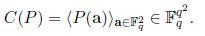
So the first co-ordinate of C(P) would have the value of P(1,1), the second coordinate would have the value of P(1,2), and in general the (i*q+j)th coordinate of C(P) would have the value P(i,j).

The rate of this code is less than 1/2 and it can be shown that the correct value at a particular coordinate of the received codeword can be decoded by making only O(√k) queries on the received codeword, assuming that a constant fraction of the codeword gets corrupted.

Multiplicity codes. The key idea in the paper is to encode the message using multivariate polynomials and their partial derivatives. If we plug this idea to the above example, each coordinate of the codeword will have 3 alphabets instead of one or in other words each coordinate would be a value from ( F_{q}^3 ). So the codeword is now:

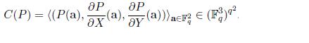
This improves the rate from <1/2 to 2/3! It can be done without increasing the query complexity. This by itself is a new result. What’s more is they can extend this idea to get codes of arbitrarily high rate while keeping the query complexity small. Here is their main theorem from the paper:

For every ε>0, α>0, and for infinitely many k, there exists a code which encodes k-bit messages with rate 1-α, and is locally decodable from some constant fraction of errors using O(k^ε) time and queries.

Umesh Vazirani. Certifiable Quantum Dice.

Background. Many computational tasks such as cryptography, game theoretic protocols, physical simulations, etc. require a source of independent random bits. But constructing a truly random device is a hard task. Even assuming that such a device is available, how do we test if it is working correctly? This task seems impossible since a perfect random number generator must output every n bit sequence with equal probability and there is no reason one can reject a particular output in favor of an other.

Quantum mechanics offers a way to get past this fundamental barrier: starting with O(log² n) random bits one can generate n certifiable random bits.

To get an idea of how this is possible let us consider the CHSH game first (given below).

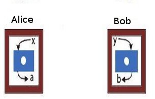The CHSH game. Alice and Bob are two co-operating players who receive inputs x and y, respectively from a third party. Alice and Bob are at two different locations. The winning condition for them is to produce outputs a and b such that the following condition is satisfied: If x=y=1, then a and b must be different. For any of the other three combinations of x and y, the outputs have to be equal. If the players are correlated according to the laws of classical physics, only any three of the four pairs of inputs can be satisfied. So the maximum probability of winning is 0.75. However, if they adopt a strategy based on quantum correlations, this value can be increased to 0.851. See the references in this article in Nature for more details.

We can define a quantum regime corresponding to the success probabilities between 0.75 and 0.85. It is simple to construct two quantum devices corresponding to any value in the regime. But if two devices produce co-relations in the regime, they must be randomized. Or in other words, randomness is for real! This gives a simple statistical test to cerfify randomness.

Result. We are using two random input bits (x,y) to produce two random output bits, so this doesn’t accomplish much. We cannot claim the output to be more random than the input. Vazirani and Vidick in their paper describe a protocol that uses O(log ² n) seed bits to produce n certifiable random bits.

Jaikumar Radhakrishnan. Communication Complexity of Multi-Party Set-Disjointness Problem.

Consider the following problem: Alice and Bob are given inputs x and y respectively and are asked to compute a function f(x,y). They are charged for the number of bits exchanged. The minimum number of bits that have to be exchanged in order to compute the function f is the communication complexity of the problem. A particular problem that is of interest in the area of communication complexity is the set-disjointness problem.

Problem. There are k parties each of whom has a subset from {1,..,n} stuck on his forehead. Each party can see the all the subsets except his own. The set-disjointness problem is to determine if the intersection of all the k subsets is empty. Again, we charge for the number of bits exchanged. All the parties have access to a shared blackboard on which they can write, so we have a broadcast medium.

The case when k=2 is well-understood both in both deterministic and randomized settings. (In randomized version, all the parties have access to a shared source of infinite random bits.)

Results. Until recently, for the general multi-party case, the best lower bound on communication complexity known for the number-on-the-forehead model was Ω(n^1/k+1/2^{k^2}). Last year, Sherstov improved this bound to Ω(n/4^k)^1/4 which is close to tight.

Jaikumar is a fantastic teacher. In what was basically a blackboard-talk, he gave an overview of the main ideas in Sherstov’s proof in a way that was accessible even to non communication-complexity experts. The arguments are based on approximating Boolean functions by polynomials.

Other talks in BTCS

There were several other good talks. Naveen Garg surveyed the recent progress on approximation algorithms for the Traveling Salesman Problem that achieve a strictly better than 1.5 approximation factor. Manindra presented the result on lower bound on ACC by Ryan Williams. Aleksender Madry gave two talks: one in which he presented a new randomized algorithm for the k-server problem that achieves poly-logarithmic competitiveness and one on approximating max-flow in capacitated, undirected graphs using the techniques from electrical flows and laplacian systems. Nisheeth Vishnoi discussed new algorithms for the Unique Games Conjecture. Amit Kumar gave a talk about a recent result by Friedman, Hansen and Zwick on proving lower bounds for randomized pivoting rules in simplex algorithm. Sanjeev Khanna spoke about some recent progress on the approximability of the edge-disjoint paths problem. Most of these results are now famous in theory-circles.

Conference talks

There were 38 papers out of which about 16 were from Theory A. Here are some of the talks I attended:

The Semi-stochastic Ski-rental Problem. (Aleksander Mądry and Debmalya Panigrahi)

An online algorithm is an algorithm which optimizes a given function when the entire input in not known in advance, but is rather revealed sequentially. The algorithm has to make irrevocable choices about the output as the input is seen. The ratio of the performance of the online algorithm to the optimal offline algorithm is called the competitive ratio of the algorithm.

On one hand, we have online models which assume nothing about the input and on the other we have stochastic models which assume that the input comes from a known distribution. The semi-stochastic model in this paper unifies these two extremes. In this model, the algorithm does not know the input distribution initially, but can learn the distribution by asking queries. The algorithm has a certain query budget. If the budget is zero (resp. infinite), the model reduces to the online (resp. stochastic) version. The goal is to maximize the competitive ratio assuming that the queries are answered adversarially.

This model is well-motivated because in many real world situations, the online model is too pessimistic and the stochastic model is too optimistic. We can usually learn the input distribution to some extent and often learning the distribution incurs some cost.

Problem. The ski-rental problem is studied in this framework. The problem is as follows: Ann wants to go skiing, but she does not know the exact number of days she would like to ski. Each morning she has to decide if she has to rent a pair of skis or buy them. Renting the skis cost 1 unit/day and buying them would cost b units. The goal is to minimize the total cost.

Here is a trivial 2-competitive algorithm: Rent the skis for b-1 days. If she decides to go on the bth day, then buy them. This is the best one can do in a deterministic setting. The best randomized algorithm gives a competitive ratio of e/(e-1).

Results. Given a desired competitive ratio e/(e-1)+ε, the paper gives lower and upper bounds on the number of queries that need to be asked in order to achieve that ratio. The lower bound is C/ε (where C is a universal constant) and the upper bound is O(1/ε^1.5).

Rainbow Connectivity: Hardness and Tractability. Prabhanjan Ananth, Meghana Nasre, and Kanthi K Sarpatwar.

Problem. In an edge-colored graph, a rainbow path is a path in which all the edges have different colors. Given a graph G, can we color the edges using k colors such that every pair of vertices has a rainbow path between them? In short, is rc(G) ≤ k? A graph is said to be rainbow connected if the above condition is satisfied. Further, for every pair, if one of the shortest paths between them is a rainbow path, then the graph is said to be strongly rainbow connected (src(G)).

Results.The paper shows that determining if src(G) ≤ k is NP-hard even for bipartite graphs. The hardness of determining if rc(G) ≤ k was open for the case when k is odd. The authors establish the hardness for this case (for every odd k≥3) by an indirect reduction from vertex coloring problem. The argument is combinatorial in nature. I’m not sure if the same argument can be tweaked for the case when k is even (which might simplify the overall proof of hardness for every k≥3.)

Simultaneously Satisfying Linear Equations Over F₂. (by Robert Crowston et. al)

Problem. We are given a set of m equations containing n variables x₁,…,x_n of the form ∏_i∈Ix_i=b. The x_is and b take values from {-1,1}. For example, equations can be x₁x₄x₈=1, x₂x₅x_n=-1, etc. Each equation is associated with a positive weight. The objective is to find an assignment of variables such that the total weight of the satisfied equations is maximized.

The problem is known to be NP-Hard, so we concentrate on a special case. Let the total weight of all the equations be W. If we randomly assign 1 or -1 to each variable, every equation gets satisfied with probability 1/2. Hence, there is always an assignment that is guaranteed to give a weight of W/2. The problem MAX-LIN[k] is to find the complexity of finding an assignment with weight W/2+k, where k is the parameter.

Roughly, a problem is said to be fixed-parameter-tractable (FPT) is if an input instance containing n input bits and an integer k (called the parameter) can be solved in time f(k)n^O(1), where f(k) depends only on the parameter k.

Results. The authors show that the problem MAX-LIN[k] is FPT and admits a kernel of size O(k² log k) and give an O(2^{O(klog k)}(nm)^c) algorithm. They also have new results for a variant of the problem where the number of variables in the equation is fixed to a constant. The results in the paper is built on the previous results by the same authors some parts of which use Fourier analysis of pseudo-Boolean functions. I’m not familiar with these techniques.

Obtaining a Bipartite Graph by Contracting Few Edges. (by Pinar Heggernes et. al)

Problem. Given a graph G, can we obtain a bipartite graph by contracting k edges? This problem though simple to state was not studied before. Which is quite surprising considering that the related problem of removing vertices to obtain a bipartite graph is a central problem in parametrized complexity.

Results. The main result of the paper shows that the problem is fixed-parameter-tractable when parametrized by k. The result makes use of many techniques well-known in parametrized complexity like iterative compression, irrelevant vertex and important separators. An interesting open question is to decide if the problem admits a polynomial kernel.

The update complexity of selection and related problems. (Manoj Gupta, Yogish Sabharwal, and Sandeep Sen)

Problem. We want to compute the function f(x₁,x₂,…,x_n) when the x_is are not known precisely but rather just known to lie in an interval. We are allowed to query and update a particular variable, to get a more refined estimate. Each query has some cost. The objective is to compute the function f with minimum number of queries.

Results. The previous literature focuses on the case when the query returns the exact value of the variable. This paper generalizes the model by allowing query updates that return open or closed intervals or points instead of exact values. The performance of the online algorithm is compared against an offline algorithm that knows the input sequence and therefore is able to ask the minimum number of queries to an adversary. For some selection problems and MST, the authors show that a 2-update competitive ratio holds for the general model.

Optimal Packed String Matching. (by Oren Ben-Kiki et. al)

Problem. Given a text containing n characters find if a string of m characters appears in the text.

Results. This is an age-old problem. The paper considers the packed string matching case where each machine word can hold up to α characters. The paper presents a new algorithm that extends the Crochemore-Perrin constant-space O(n) algorithm to run get an O(n/α) algorithm. Thus achieving a speed-up of factor α. The packed string matching problem is also-well studied. What is different in this paper is that they achieve better running times by assuming two instructions that have become recently available on processors: one is string-matching instruction WSSM which can find a word of size α in a string of size 2α and the other is WSLM instruction which can find the lexicographically maximal-suffix in a word.

Physical limits of communication. (Invited talk by Madhu Sudan)

Given a piece of copper wire, what is stopping us from transmitting infinite number of bits in unit time on it? The is a fundamental question in communication theory. There could be two reasons why the capacity could be unbounded. Firstly, the signal strength is a real value so there are infinite number of them. Secondly, there are infinitely many instances of time at which a signal can be sent. The first possibility is ruled out due to the presence of noise. It appears that the delay in transmission time rules out the second possibility too, but this has not been extensively studied.

This paper studies this problem in a model where the communicating parties can divide the time into any number of slots but have to cope up with (possibly macroscopic) delays. The surprising result is that the capacity of the channel is bounded only when either noise or delay is adversarially chosen. If both the error sources are stochastic (or if noise is adversarial but independent of stochastic delay) then the capacity of the channel is infinite!

There were other invited talks by Susanne Albers, Moshe Vardi, John Mitchell, Phokion Kolaitis and Umesh Vazirani. Unfortunately, I missed many of these talks.

On the lighter side

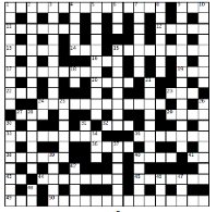
TCS Crossword

Try these:

• A confluence of researchers that generates fizz? (4)
• Fundamental fight (6,4)
• If the marking is right, it will fire! (8)

Find more clues like these and the grid in the TCS Crossword that was handed out to attendees during a coffee-break.

Algorithmic Contest (for students)

There was an algorithmic-contest as part of the conference (hosted on Algo Muse). Here is a take-away puzzle:

Contiguous t-sum problem. Given an array A[1..n] and a number t as input, find out if there exists a sub-array whose sum is t. For example, if the input is the array shown below and t=8, the answer is YES since A contains the sub-array A[2..4] whose sum is t. Prove an Ω(n log n) lower bound for the above problem on a comparison model.

Many CSTheory people probably know there is a new StackExchange Q&A site, Theoretical Physics, which is now in public beta, and was originally started by Joe Fitzsimons, co-editor of this blog.  My purpose for this post is to give TCS people a heads-up that there are now 16 questions on that site under the quantum-computing tag and the quantum-information tag that may be of interest to theoretical computer science.

My favorite of these questions is Rigorous Security Proof for Wiesner’s Quantum Money?  In this question, Scott Aaronson asks for an explicit upper bound on a value that is “known to exist” according to folklore, but that he and a co-author were unable to find in the literature or derive. Master’s student Abel Molina solves the problem, using a formalism of Gutoski and Watrous.  John Watrous then verifies the solution’s correctness.  There are also contributions by Dan Gottesman and Peter Shor.

In related news, there is now a proposal for a Quantum Information question and answer site on the Stack Exchange Area 51.  This proposal is (mildly) controversial, though, because some people are concerned it would duplicate topics already available on Theoretical Physics.

Are some questions harder than others?

Last time we quantified hardness of answering a question with a quantum computer as the quantum query complexity. We promised that this model would allow us to develop techniques for proving lower bounds. In fact, in this model there are two popular tools: the polynomial method, and the (negative) adversary method.

The original version of the quantum adversary method, was proposed by Ambainis [Amb00]. The method starts by choosing two sets of inputs on which \(f\) takes different values. Then the lower bound is determined by combinatorial properties of the graph of the chosen inputs. Some functions, such as sorting or ordered search, could not be satisfactorily lower-bounded by the unweighted adversary method. Hoyer, Neerbek, and Shi [HNS02] weighted the input pairs and obtained the lower bound by evaluating the spectral norm of the Hilbert matrix. Barnum, Saks, and Szegedy [BSS03] proposed a complex general method and described a special case, the spectral method, which gives a lower bound in terms of spectral norms of an adversary matrix. Ambainis also published a weighted version of his adversary method [Amb03]. He showed that it is stronger than the unweighted method but this method is slightly harder to apply, because it requires one to design a weight scheme, which is a quantum counterpart of the classical hard distribution on inputs. Zhang [Zha05] observed that Ambainis had generalized his oldest method in two independent ways, so he united them, and published a strong weighted adversary method. Finally, Laplante and Magniez [LM04] used Kolmogorov complexity in an unusual way and described a Kolmogorov complexity method. Spalek and Szegedy [SS06] unified the above methods into one equivalent method that can be formulated as a semidefinite program (SDP).

We will present an alternative development observed by Reichardt in terms of optimization problems [Rei11]. Our approach will use SDP duality extensively, but we will not prove the duals explicitly, referring the interested reader to previous literature instead [SS06, Rei09].

From certificate complexity to the adversary method

The certificate complexity of a function \(f\) is the non-deterministic version of query complexity and can be found by solving the following optimization problem:

\[ \begin{aligned} C(f) & = \min_{\vec{p}_x \in \{0,1\}^n} \max_x ||\vec{p}_x||^2 \\ \text{s.t.} & \sum_{j:x_j \neq y_j} p_x[j]p_y[j] \geq 1 \quad \text{if} \; f(x) \neq f(y) \end{aligned} \]

We think of \(\vec{p}_x\) as a bit-vector with the \(j\)-th component telling us if index \(j\) is in the certificate or not. The constraint is simply the contrapositive of the definition of certificate complexity: if \(f(x) \neq f(y)\) then there must be at least one bit of overlap on the certificates of \(x\) and \(y\) such that they differ on that bit. The discrete nature of the bit-vector makes certificate complexity a difficult optimization, and it is natural to consider a relaxation:

\[ \begin{aligned} Adv^*(f) & = \min_{\vec{p}_x \in \mathbb{R}^n} \max_x ||\vec{p}_x||^2 \\ \text{s.t.} & \sum_{j:x_j \neq y_j} p_x[j]p_y[j] \geq 1 \quad \text{if} \; f(x) \neq f(y) \end{aligned} \]

Note the suggestive name: the above equation corresponds to the dual of the adversary method. Its more common form is the primal version:

\[ \begin{aligned} Adv(f) & = \max_{\Gamma \in \mathbb{R}^{|D| \times |D|}} ||\Gamma|| \\ \text{s.t.} & \forall j \quad ||\Gamma \cdot \sum_{x,y:x_j \neq y_j} |x\rangle\langle y | || \leq 1 \\ & \Gamma[x,y] = 0 \quad \text{if} \; f(x) = f(y) \\ & \Gamma[x,y] \geq 0 \end{aligned} \]

Since the adversary bound is a relaxation of the certificate complexity, we know that \(Adv(f) \leq C(f)\) for all \(f\). In fact, two even stronger barrier stands in the way of the adversary method: the certificate and property testing barriers. The certificate barrier is that for all functions \(f\), \(Adv(f) \leq \min { \sqrt{C_0(f)n}, \sqrt{C_1(f)n} }\), and if \(f\) is total, then we have \(Adv(f) \leq \sqrt{C_0(f) C_1(f)}\) [Zha05, SS06]. The property testing barrier is for partial functions, where every zero-input is of Hamming distance at least \(\epsilon n\) from every one-input. In that case the method does not yield a lower bound better than \(1/\epsilon\).

Negative adversary method

To overcome these barriers, Hoyer, Lee, and Spalek [HLS07] introduced the negative adversary method. The method is a relaxation of the adversary method that allows negative weights in the adversary matrix:

\[ \begin{aligned} Adv^{\pm}(f) & = \max_{\Gamma \in \mathbb{R}^{|D| \times |D|}} ||\Gamma|| \\ \text{s.t.} & \forall j \quad ||\Gamma \cdot \sum_{x,y:x_j \neq y_j} |x\rangle\langle y | || \leq 1 \\ & \Gamma[x,y] = 0 \quad \text{if} \; f(x) = f(y) \end{aligned} \]

Note that we started with certificate complexity and relaxed that to get the dual of the adversary method. We took the dual to get the adversary method, and then relaxed the adversary method to get the negative adversary method. Since we relaxed in both directions in two different ways, the negative adversary method is not clearly related to the certificate complexity.

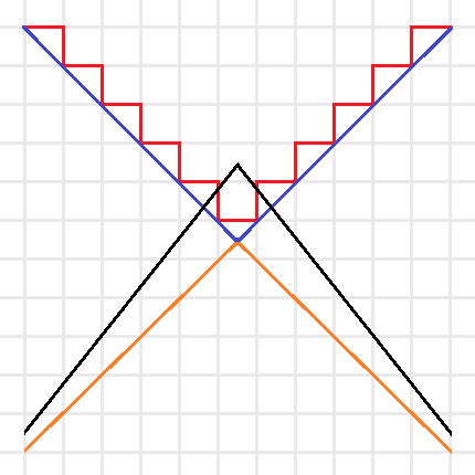
Intuitive sketch of the optimization problems for \(C(f)\) (Red), \(Adv^*(f)\) (Blue), \(Adv(f)\) (Orange), and \(Adv^\pm(f)\) (Black). Note that the red and blue lines are the boundaries of minimization problems, thus their feasible regions are above the boundaries, and the orange and black lines are the boundaries of maximization problems, thus their feasible regions are below the boundaries.

We can simplify this idea with the above picture. The certificate complexity involved a minimization over the integers, so its feasible region is above the boundary drawn by the red line. The optimization problem for \(C(f)\) tries to find the lowest point in the feasible region. The adversary method replaces the integer constraint by real values, and is represented by the blue line. Since the optimization of \(Adv^*(f)\) is still a minimization, this allows us to find lower points in the bigger feasible region. Since the goal of the method is to provide a lower bound, we instead look at \(Adv(f)\) as a maximization problem (with boundary in orange), now the feasible region is below the orange line and any feasible point provides a lower bound. Note that by duality this lower bound is always less than or equal to a feasible point in \(Adv^*(f)\)’s region and thus less than or equal to the certificate complexity. The negative adversary method’s feasible region is represented by the black line. It takes the maximization in \(Adv(f)\) and removes the non-negativity constraint, expanding the feasible region and thus making it possible to find points with \(Adv^\pm(f) > Adv(f)\). Finding natural problems where we have a separation though, has proved to be difficult. In particular, for important problems beyond the certificate complexity barrier (like the collision problem) our best lower bounds come from the polynomial method, and no one has found an approach that uses the negative adversary method directly. Do you know a natural \(f\) such that \(Adv^\pm(f) > Adv(f)\) or better yet, such that \(Adv^\pm(f) > C(f)\)?

Query complexity and the negative adversary method

Of course, without context the method is not very useful. It is the fact that it lower bounds quantum query complexity that first made it a useful tool. Given a function \(f: D \subseteq \{0,1\}^n \rightarrow \{0,1\}\), we have:

\[ Q_\epsilon(f) \geq \frac{1 – 2\sqrt{\epsilon(1 – \epsilon)}}{2} Adv^{\pm}(f) \]

To prove this relation, we think of an adversary holding a quantum superposition \(|\delta\rangle\) over oracle strings instead of the oracle representing a specific input. This \(|\delta\rangle\) is found by the negative adversary method, and corresponds to any eigenvalue of \(\Gamma\) with eigenvalue \(||\Gamma||\). Thus, any algorithm for solving the problem starts with the initial state (refer to the query complexity post for background on notation):

\[ |\Psi_0\rangle = \delta_x |x\rangle_I \otimes |1,0\rangle_Q |0\rangle_W \]

We then consider the reduced density matrix \(\rho_t = Tr_I |\Psi_t\rangle\langle \Psi_t |\) that the adversary holds. This state begins with no entanglement, and in order to learn \(x\) we must create a lot of entanglement in the state. Specifically, we define a progress function \(W^t = \langle \Gamma, \rho_t \rangle\) and show 3 points:

1. \(W^0 = ||\Gamma||\).
2. \(W^t – W^{t+1} \leq 2 \max_j ||\Gamma \cdot \sum_{x,y:x_j \neq y_j} |x\rangle\langle y | ||\)
3. \(W^T = 2\sqrt{\epsilon(1 – \epsilon}||\Gamma||\)

The first step is obvious from our choice of the adversary’s initial state and progress function. The second step is an application of Cauchy–Schwarz and triangle inequalities. The third-step demands that the algorithm give the correct output: \(||\Pi_{f(x)} |\psi_x^T\rangle ||^2 \geq 1 – \epsilon\). This is the most difficult step, and the proof goes through a few special choices of operators and an application of Holder’s inequality. We reference the reader to the original paper [HLS07] for details.

Where do we go from here?

Does the negative adversary method answer if some questions are harder than others? Next time we will see that by looking at span program we can show that the negative adversary method characterizes query complexity: \(Q(f) = \Theta(Adv^\pm(f))\). Thus, the method is a great way to show that some questions are more difficult than others. It also behaves well with respect to iterated functions. In particular, to break the certificate complexity barrier, we can iterate the Kushilevitz-Ambainus partial function \(f\) on 6 bits, defined as:

• Zero inputs of \(f\) are: \( 111000, 011100, 001110, 100110, 110010, 101001, 010101, 001011, 100101, 010011\),
• One inputs of \(f\) are: \( 000111, 100011, 110001, 011001, 001101, 010110, 101010, 110100, 011010, 101100\).

We leave it as an exercise to the eager reader to use their favorite SDP solver to show that \( Adv^\pm(f) \geq 2 + 3\sqrt{5}/5 > C(f) = 3\).

References

[Amb00] A. Ambainis. Quantum lower bounds by quantum arguments. In Proceedings of the thirty-second annual ACM symposium on Theory of computing, pages 636-643. ACM, 2000, arXiv:quant-ph/0002066v1.

[Amb03] A. Ambainis. Polynomial degree vs. quantum query complexity. In Foundations of Computer Science, 2003. Proceedings. 44th Annual IEEE Symposium on, pages 230{239. IEEE, 2003, arXiv:quant-ph/0305028.

[BSS03] H. Barnum, M. Saks, and M. Szegedy. Quantum decision trees and semidefinite programming. In Proc. of 18th IEEE Complexity, pages 179-193, 2003.

[HLS07] Peter Hoyer, Troy Lee, and Robert Spalek. Negative weights make adversaries stronger. 2007, arXiv:quant-ph/0611054v2.

[HNS02] P. Hoyer, J. Neerbek, and Y. Shi. Quantum complexities of ordered searching, sorting, and element distinctness. Algorithmica, 34(4):429-448, 2002, arXiv:quant-ph/0102078.

[LM04] S. Laplante and F. Magniez. Lower bounds for randomized and quantum query complexity using Kolmogorov arguments. 2004, arXiv:quant-ph/0311189.

[Rei09] Ben W. Reichardt. Span programs and quantum query complexity: The general adversary bound is nearly tight for every boolean function. In 2009 50th Annual IEEE Symposium on Foundations of Computer Science, pages 544-551. IEEE, 2009, arXiv:0904.2759v1 [quant-ph].

[Rei11] Ben W. Reichardt. Quantum query complexity. Tutorial at QIP2011 Singapore, 2011.

[SS06] Robert Spalek and Mario Szegedy. All quantum adversary methods are equivalent. Theory of Computing, 2:1-18, 2006, arXiv:quant-ph/0409116v3.

[Zha05] S. Zhang. On the power of Ambainis lower bounds. Theoretical Computer Science, 339(2-3):241-256, 2005, arXiv:quant-ph/0311060.

How hard is it to answer a question? As theoretical computer scientists, this query haunts us. We formalize a ‘question’ as a function on some input and ‘answering’ as running a finite procedure. This procedure might run on a Turing Machine, your cellphone, or a quantum computer. ‘Hard’ is quantified by use of resources such as energy, space or time. Unfortunately, the most popular notion of hardness — time complexity — is notoriously difficult to characterize in a quantum computing model. If we want to show what a model of computation can and can’t do, we must use a related, but simpler measure of complexity. For quantum computing this measure is quantum query complexity. This post explains quantum query complexity and lays the foundations for future entries that will introduce the lower bound technique of the (negative) adversary method, and show how it characterizes quantum query complexity through its connection to span programs.

In the query model, the input to our algorithm is given as a black-box (called the oracle). We can only gain knowledge about the input by asking the oracle for individual bits. The input is a bit-string \( x \in D \subseteq \{0, 1\}^n \) and the goal is to compute some function \(f : D \rightarrow \{0,1\}\). If \(D = \{0,1\}^n\) then we call the function total. For simplicity, we only consider decision problems (binary range), although the machinery has been developed for functions over finite strings in arbitrary finite input and output alphabets.

The query complexity of a function is the minimum number of queries used by any circuit computing the function. For a two-sided error \(\epsilon\), we denote the query complexity by \(Q_\epsilon(f)\). Since success amplification is straightforward, we abbreviate further by setting \(Q(f) = Q_{1/3}(f)\). Similar measures exist for classical algorithms, where this model is more frequently referred to as decision-tree complexity. The usual notation is \(D(f)\) for deterministic query complexity, \(R(f)\) for two-sided error (\(1/3\)) randomized query complexity, and \(C(f)\) for certificate (or non-deterministic) complexity. We specify our model concretely, following [HS05]:

Quantum query model: formally

The memory of a quantum query algorithm is described by three Hilbert spaces (registers): the input register, \(H_I\), which holds the input \(x \in D\), the query register, \(H_Q\), which holds an integer \(1 \leq i \leq n\) and a bit \(b \in \{0,1\}\), and the working memory, \(H_W\), which holds an arbitrary value. The query register and working memory together form the memory accessible to the algorithm, denoted \(H_A\). The unitaries that define the algorithm can only act on this space. The accessible memory of a quantum query algorithm is initialized to a fixed state. On input \(x\) the initial state of the algorithm is \(|x\rangle_I \otimes |1, 0\rangle_Q \otimes |0\rangle_W\). The state of the algorithm then evolves through queries, which depend on the input register, and accessible memory operators which do not.

A query is a unitary operator where the oracle answer is given in the phase. We definite the operator \(O\) by its action on the basis state \(|x\rangle_I \otimes |i,b\rangle_Q\) as

\[ O |x\rangle_I \otimes |i,b\rangle_Q = (-1)^{bx_i} |x\rangle_I \otimes |i,b\rangle_Q \]

The accessible memory operator is an arbitrary unitary operation \(U\) on the accessible memory \(H_A\). This operation is extended to act on the whole space by interpreting it as \(I_I \otimes U\) and \(O\) is interpreted as \(O \otimes I_W\). Thus the state of the algorithm on input \(x\) after \(t\) queries can be written as:

\[ |x\rangle_I |\psi^t_x\rangle_A = U_t O U_{t-1} … U_1 O U_0 |x\rangle_I |1, 0\rangle_Q |0\rangle_W \]

Where we noticed that the input register is left unchanged by the algorithm. The output of a \(T\)-query algorithm is distributed according to the state of the accessible memory \(|\psi^T_x\rangle\) and two projections \(\Pi_0\) and \(\Pi_1\) such that \(\Pi_0 + \Pi_1 = I\) corresponding to the possible outcomes of a decision problem. The probability that given input \(x\) the algorithm returns \(0\) is \(||\Pi_0|\psi^T_x\rangle||^2\) and \(1\) is \(||\Pi_1|\psi^T_x\rangle||^2\). \(Q_\epsilon(f)\) is the minimum number of queries made by an algorithm which outputs \(f(x)\) with probability \(1 – \epsilon\) for every \(x\).

Relations between models

For partial functions, the quantum query complexity can be exponentially smaller than randomized or deterministic query complexity [Sho95, BV97, Sim97, Aar10]. However, if the partial function is invariant under permuting inputs and outputs then the complexities are polynomially related with \(R(f) = O(Q(f)^9)\) [AA09]. If the function is total, then \(D(f)\) is bounded by \(O(Q(f)^6)\) , \(O(Q(f)^4)\) for monotone total functions, and \(O(Q(f)^2)\) for symmetric total functions [BBC+01]. However, no greater than quadratic separations are known for total functions (this separation is achieved by \(OR\), for example). This has led to the conjecture that for total functions \(D(f) = O(Q(f)^2)\). This conjecture is open for all classes of total functions, except monotone [BBC+01], read-once [BS04], and constant-sized 1-certificate functions.

The infamous time complexity is always at least as large as the query complexity since each query takes one unit step. For famous algorithms such as Grover’s search [Gro96] and Shor’s period finding (which is the quantum part of his famed polynomial time factoring algorithm) [Sho95], the time complexity is within poly-logarithmic factors of the query complexity. There are also exceptions to the tight correspondence. The Hidden Subgroup Problem has polynomial query complexity [EHK04], yet polynomial time algorithms are not known for the problem.

By taking the computation between queries as free, we get a handle for producing lower bounds. This allows us to develop strong information-theoretic techniques for lower bounding quantum query complexity. In my next post I will use this framework to develop the (negative) adversary method.

References

[AA09] Scott Aaronson and Andris Ambainis. The need for structure in quantum speedups. 2009, arXiv:0911.0996v1 [quant-ph].

[Aar10] Scott Aaronson. BQP and the polynomial hierarchy. In Proceedings of the 42nd ACM symposium on Theory of computing, pages 141-150. ACM, 2010, arXiv:0910.4698 [quant-ph].

[BBC+01] R. Beals, H. Buhrman, R. Cleve, M. Mosca, and R. de Wolf. Quantum lower bounds by polynomials. Journal of the ACM (JACM), 48(4):778-797, 2001.

[BS04] H. Barnum, and M. Saks. A lower bound on the quantum query complexity of read-once functions. Journal of Computer and System Sciences, 69(2):244-258, 2004. arXiv:quant-ph/0201007v1

[BV97] E. Bernstein and U. Vazirani. Quantum complexity theory. SIAM J. Comput., 26(5):1411-1473, 1997.

[EHK04] M. Ettinger, P. Hoyer, and E. Knill. The quantum query complexity of the hidden subgroup problem is polynomial. Information Processing Letters, 91(1):43-48, 2004, arXiv:quant-ph/0401083v1.

[Gro96] L.K. Grover. A fast quantum mechanical algorithm for database search. In Proceedings of the twenty-eighth annual ACM symposium on Theory of computing, pages 212-219. ACM, 1996, arXiv:quant-ph/9605043.

[HS05] P. Hoyer, and R. Spalek. Lower Bounds on Quantum Query Complexity. Bulletin of the European Association for Theoretical Computer Science, 87, 2005. arXiv:quant-ph/0509153v1.

[Sim97] D.R. Simon. On the power of quantum computation. SIAM Journal on Computing, 26:1474, 1997.

[Sho95] P.W. Shor. Polynomial-time algorithms for prime factorization and discrete logarithms on a quantum computer. SIAM J. Comput., 26:1484-1509, 1995, arXiv:quant-ph/9508027.