I saw a nice result sketched a few weeks ago, on the “online matching” problem. Below I try to re-explain the result, using some idiomatic (and as a bonus, inoffensive) terminology which I find makes it easier to remember what’s going on.

Online Matching. There is a set of items, call them Lunches, which you want to get eaten. There is a set of people who will arrive in a sequence, call them Diners. Each Diner is willing to eat certain Lunches but not others. Once a Diner shows up, you can give them any remaining Lunch they like, but that Lunch cannot be re-sold again. The prototypical problem is that a Diner might show up but you already sold all of the Lunches that they like. Your task: find a (randomized) strategy to maximize the (expected) number of Lunches sold, relative to the maximum Lunch-Diner matching size.

This is an online problem: you don’t have all the information about Diner preferences before the algorithm begins, and you need to start committing to decisions before you know everyone’s preferences in full.

Consider the following strategy:

Algorithm: pick a random ordering/permutation of the lunches; then when a diner arrives, give her the first available lunch in the ordering that she likes.

How does this perform? In expectation at least (1-1/e)M lunches are sold, where M is the maximum (offline) matching size in the Lunch-Diner graph. But proving so is tricky. (This ratio 1-1/e turns out to be the best possible.) Birnbaum and Mathieu recently gave a simpler proof that this ratio is achieved. Amin Saberi, whose talk sketched this, rightly pointed out that it feels like a “proof from The Book!”

With a small lemma (e.g. Lemma 2 in Birnbaum-Mathieu), we may assume that the number of diners and lunches are equal, and that there is a perfect matching between diners and lunches. Let the number of diners and lunches each be n, and so M=n.

Let x_t be the probability that in a random lunch permutation, upon running Algorithm, the lunch in position t is eaten.

Experiment 1. Take a random lunch permutation. Score 1 if the lunch at position t is not eaten, 0 if it is eaten. The expected value of this experiment is 1-x_t.

Experiment 2. Take a random lunch permutation, and a random diner. Score 1 if that diner eats a lunch in one of the first t positions, 0 otherwise. The expected value of this experiment is (x₁ + … + x_t)/n.

The key is to show that the second experiment has expected value greater than or equal to the first one, then we will finish up by an easy calculation. We do this with a joint experiment, similar to “coupling” arguments.

Joint experiment. Let t be fixed. Take a random lunch permutation π₁, and look at the lunch L in position t. Let D be matched to L in the perfect matching. Obtain π₂ from π₁ by removing L and re-inserting L in a random position.

Key claim: π₂ and D are independent, uniformly distributed random variables. This implies that we can run both experiments at the same time using this joint distribution on π₁, π₂, L, D. Moreover,

Deterministic Lemma. For any π₁, and for an uneaten lunch L at position t in π₁, obtain π₂ from π₁ by removing L and re-inserting L in any position. Let D be matched to L in the perfect matching. Then in π₂, D eats one of the first t lunches.

This implies that whenever experiment 1 scores a point, so does experiment 2. So taking expectations,

(x₁ + … + x_t)/n ≥ 1-x_t.

This equation is the crux. Let x_≤t = x₁+…+x_t, then we see x_≤t ≥ (ⁿ/_n+1)(1+x_≤t-1). This recursion is easy to unravel and it gives a lower bound of n(1-(ⁿ/_n+1)ⁿ) ≥ n(1-1/e) on x_≤n, the expected size of the matching!

(This is a cross-post from my blog, which has posts commonly on math and/or lunches.)

There is a new page to this blog: Theoretical Computer Science Conferences and Workshops.  It provides names and links to theory venues — with theory broadly defined, including, for example, the theory of programming languages, which is usually considered outside the SIGACT purview  (EDIT: see comments).  This page is the result of dozens of contributions to a community wiki question on CSTheory, and Joe and I would like to thank everyone who participated.

Those interested in lists of TCS venues may also want to check out Microsoft Research’s list of computer science conferences.  That list considers all of CS, not just theory, and provides some added information, like citations per conference.  The list on this blog contains some conferences that the MR list does not.

If you see errors, or can think of useful additions, please comment here or on the new page, or edit the community wiki answer that contains the conference information.  Thanks, and we hope you find this helpful.

Almost exactly one year ago (10 Sept 2010), Cem Say asked the following deceptively simple question:

Is the language $latex \{ a^{i}b^{j}c^{k} \mid  i \neq j, i \neq k, j \neq k \}$ non-context-free?

Recall that a language is context-free if it can be accepted by a pushdown automaton.  A pushdown automaton, in turn, is a finite automaton with access to a stack (so it has access to an unbounded amount of memory).  A standard example of a context-free language that cannot be recognized by a finite automaton without a stack is {$latex a^n b^n \mid n \geq 1 $}.  If a finite automaton has no access to a stack, it cannot store the value of $latex n$ if $latex n$ gets too large, so it has no way to be certain that the number of $latex b$ appearing exactly match the number of $latex a$.  This intuition is formalized in the famous pumping lemma; and there is a similar tool, the pumping lemma for context-free languages, that can be used to prove that a language is not context-free.

It is easy to apply a standard technique — the pumping lemma — to show the language Cem Say asked about is not regular.  (We make the exponents large enough that a finite automaton has to repeat a state, and take advantage of that confusion.)  However, there doesn’t appear to be a good way to apply the pumping lemma for context-free languages to show this particular language is context-free.  Initially, though, some site members thought the question was easy enough to be undergraduate homework, since the definition of the language is so close to other languages whose status can be resolved with a pumping lemma.

Fortunately, Frank Weinberg knew about Ogden’s Lemma, which is an extension of the pumping lemma for context-free languages (the pumping lemma is a special case of Ogden’s Lemma).  With this tool, he was able to prove that, indeed, the language Cem Say asked about is not context-free.  The proof I will give in this blog entry can be found in Frank Weinberg’s answer; I will give a version of the proof polished by Tsuyoshi Ito in the comments to that answer.

First, here is a statement of Ogden’s Lemma.

 Ogden’s Lemma: If $latex L$ is a context-free language, then there exists some number $latex p>0$ such that for any string $latex w$ of length at least $latex p$ in $latex L$, and every way of “marking” $latex p$ or more of the positions in $latex w$, $latex w$ can be written as $latex w=uxyzv$ with string $latex u$, $latex x$, $latex y$, $latex z$, $latex v$, such that

1. $latex xz$ has at least one marked position,
2. $latex xyz$ has at most $latex p$ marked positions, and
3. $latex ux^iyz^iv$ is in $latex L$ for every $latex i \geq 0$.

The pumping lemma for context-free languages is the special case where every position is marked.  Armed with this tool, we can now prove that $latex \lbrace a^{i}b^{j}c^{k} \mid  i \neq j, i \neq k, j \neq k \rbrace$ is not context-free.

Proof (that Cem Say’s language is not context-free): For a given $latex p$, choose $latex a^i b^p c^k$ and mark all the $latex b$’s (and nothing else).  We choose $latex i$ and $latex k$ such that for every choice of how many $latex b$’s are actually pumped there is one pumping exponent such that the number of $latex b$’s is equal to $latex i$ and one where it is equal to $latex k$.  Then $latex i$ and $latex k$ have to be from the set $latex S= \bigcap_{1 \leq n \leq p} \lbrace p-n + m*n \mid m \in IN_0\rbrace$ where $latex IN_0$ is the set of positive integers.  The set $latex S$ is infinite, because it contains $latex p+ im$ for all $latex i \geq 0$, where $latex m$ is the least common muiltiple of $latex \lbrace 1, \ldots, p \rbrace$.  So, assuming the language is context-free, we can always find an $latex i$ and $latex k$ in $latex S$ for any $latex b$, and by condition (3) of Ogden’s Lemma, the resulting string will be in $latex L$, contradicting the original definition of $latex L$.  So the language cannot be context-free after all.

For questions and answers on related topics, click on the formal languages tag.

From August 28 to September 7 I participated in the following three meetings:

1. The 6th EuroComb, in Budapest. This conference happens every 2nd year. There were 5 days, 4 parallel sessions, and discrete mathematics of every flavour, especially graphs, randomness, geometry, set systems, and algorithms.
2. Gyula Katona’s 70th birthday conference, also in Budapest at the Renyi institute.
3. The 19th European Symposium on Algorithms, in Saarbrucken. This was 3 days, with 2 parallel sessions plus more for satellite conferences, and the algorithmic topics included approximation algorithms, parameterized complexity, strings, geometry, graphs, SAT, and practical experimental work.
4. (Saarbrucken continued with two more days of the ALGO meta-conference, including ATMOS, WAOA, IPEC, and AlgoSensors. I usually attend WAOA, but this year after seeing about 80 talks in 10 days, I left for home.)

EuroComb

Here is a little bit of info about the conference. EuroComb has a small level of refereeing, allowing people to present anything, including results already published elsewhere. It was a very social conference, and this reminded me of other rarer-than-annual conferences like ISMP and CANADAM. You get to meet many people, and they generally present their best recent results, which I liked. There were a lot of people of PhD/PostDoc age but also a lot of professors, and there were participants from all over the world. (It was even a nice chance for me to make a few new acquaintances from Canadian universities.) I talked about a paper in the realm of discrete geometry that used computational methods, joint with Filip Morić.

One major plenary was given by Nets Hawk Kats. He and Larry Guth recently solved* Erdős’ distinct distances problem: show that for any n points in the plane, the number of distinct distances among these points is at least Ω(n/√log n). The * is because they only got Ω(n/log n), still it improves polynomially on all previous bounds. I have heard some discussion of the result and its proof, overall it is elegant, although the talk was not well-prepared.

In more algorithmic news, Dan Král won a major award and his plenary talk was mostly about his work on fast algorithms for variants of small-treewidth problems, extending Courcelle’s work on FOL/MSOL languages expressing very general problems that can be solved in such families. David Conlon also won the same award, and his talk was about better understanding of the tower and “wowzer” functions arising in proofs of the Szémeredi Regularity Lemma and relatives (e.g., the Graph Removal Lemma). I learned that while the tower function is T(k) = 2^(2^…^(2^2)…) where k 2’s appear, the wowzer function is W(k) = T(T(…T(2)…)) where there are k T’s.

Several interesting open problems arose at EuroComb, and here is one of them.  The rainbow colouring number of a graph is the minimum number of colours one needs to apply to the edges, so that all pairs of vertices are connected by a rainbow path (no repeated colours). Is there a constant-factor approximation for the rainbow connection number? The concept was defined only a few years ago but there have been an explosive number of papers on the topic.

Another highlight: Ken-ichi Kawarabayashi put his cat on one of his slides.

Katona 70

There is a strong tradition of birthday conferences for researchers in Budapest and apparently Gyula Katona was even one of the forces behind this tradition; his friends had a lot of very nice things to say and presents to give him. For example, he received an Indian decoration usually reserved for elephants. He is perhaps most famous for the Kruskal-Katona theorem and indeed, the majority of talks were about extremal problems in hypergraphs. My former EPFL colleague Dömötör Pálvölgyi gave a very entertaining talk about determining max/min elements with a lie: it takes about n*87/32 queries and this crazy number is tight. From another talk by Alex Sidorenko I learned a nice trick which gave me some intuition about “virtual valuations” in algorithmic game theory, which I have posted on my blog.

ESA

This is my 4th year in a row attending ESA, and it is one of my favourite conferences because many talks are about work that can be explained to a general algorithmic audience. This year, for the first time, they have given each person a USB key with electronic proceedings, which are truly awesome; not simply a .pdf dump, but a fantastic browser-navigable html/pdf hybrid.

The best paper went to Nikhil Bansal and Joel Spencer for work on a deterministic version of Spencer’s “6 Standard Deviations Suffice” work on discrepancy. This is the 2nd year in a row the best paper went to an approximation-algorithms paper, which may not be so much of a surprise given that it’s also the 2nd year in a row it went to a paper co-authored by Nikhil.

The business meeting was unusual, despite (unlike some previous years) the absence of beer. There was one serious proposal for ESA 2013, in Sophia-Antipolis, France, and one half-joking proposal in Muscat, Oman. The presenter of the latter moved there last week and basically just wanted to ensure there was some “choice” for the voters (he admitted as much and also had no price estimates). The constituency picked France over Oman by a 33-22 vote but I would not say it was a close call as everyone could see how everyone voted and some people seemed to vote just to make the vote closer. I’m not sure if it was a useful exercise since it made the business meeting non-trivially longer. It is hard to find people willing to host conferences and I am glad the final result was the one I preferred. Vive là France!

From a technical perspective, I really liked a few talks in different areas:

1. a result about MAX-SAT (out of 5 total in ALGO!) by Roth, Azar, and Gamzu since it showed naturally a matroid arising out of nowhere,
2. a constructive algorithm for “ray shooting depth” by Ray (who gave the talk and avoided making the obvious joke), Mustafa, and Shabbir, which is a plane geometry problem which previously had only a non-constructive topological proof,
3. the best student paper which was by Gawrychowski on text searching in compressed files,
4. a paper by Verschae and Wiese about scheduling unrelated machines, giving an elegant integrality gap construction and a simpler version of an existing algorithmic result from FOCS 2009,
5. nice approximation results in a model of graph vehicle routing by Schupbach and Zenklusen,
6. a talk by Justin Ward (joint w/ Feldman, Naor, Schwartz) explaining/improving many local search algorithms… for me it finally made clear what’s special about claw-free graphs.

In previous posts about graph minors, we reviewed the definitions of graph minors and topological minors, then looked at a relationship between the two; and explored whether there was a relationship between the computational hardness of a set of forbidden subgraphs and the graph class defined as all graphs that avoid the set of forbidden subgraphs.  Both of those questions are fundamentally related to the Graph Minor Theorem of Robertson and Seymour.  Today, I’d like to take a step back and look big-picture at the Graph Minor Theorem, and its relationship to computer science, by featuring an answer Timothy Chow gave to a question Ryan Williams asked about the role of the Axiom of Choice in TCS.

Ryan’s question, which he asked in October 2010, was, “What interesting theorems in TCS rely on the Axiom of Choice (or, alternatively the Axiom of Determinacy)?” The Axiom of Choice, of course, is a (sometimes controversial) axiom extending Zermelo-Fraenkel set theory, and at this point is generally accepted as part of the foundations of mathematics.  Intuitively, the Axiom of Choice says that anytime you have a mathematical construction in which there is a set of nonempty bins, then it is legal to produce a set that contains exactly one item from each bin.  While this might seem “obviously true,” once this intuition is applied to infinitely-many bins, there are nonconstructive and perhaps counter intuitive consequences.  So it is natural to wonder, in the world of TCS where the sets of bins we encounter are unlikely to be “pathologically infinite,” whether we really need the Axiom of Choice to prove anything.  (I won’t discuss the Axiom of Determinacy, except to say that it is consistent with the Zermelo-Fraenkel axioms, but inconsistent with the Axiom of Choice, and set theorists sometimes put it forth as a “better” axiom, but it has not been widely accepted by mathematicians outside of logic.)

Janne Korhonen answered Ryan’s question by noting that the proof of the Graph Minor Theorem fundamentally uses Kruskal’s Tree Theorem, which in turn uses the Axiom of Choice.  A fine answer, and one might think that was the end of the story — but one would be wrong, as Timothy Chow demonstrated in a followup answer which I will now quote from.

What about arithmetical statements whose proof requires something like Koenig’s lemma or Kruskal’s tree theorem? Don’t these require a weak form of the axiom of choice? The answer is that it depends on exactly how you state the result in question. For example, if you state the graph minor theorem in the form, “given any infinite set of unlabeled graphs, there must exist two of them such that one is a minor of the other,” then some amount of choice is needed to march through your infinite set of data, picking out vertices, subgraphs, etc. However, if instead you write down a particular encoding by natural numbers of the minor relation on labeled finite graphs, and phrase the graph minor theorem as a statement about this particular partial order, then the statement becomes arithmetical and doesn’t require AC in the proof.

So the question comes down to, “What do we really mean in theoretical computer science when we talk about a mathematical proof of an infinitary statement?”  To quote from Chow’s answer again:

Most people feel that the “combinatorial essence” of the graph minor theorem is already captured by the version that fixes a particular encoding, and that the need to invoke AC to label everything, in the event that you’re presented with the general set-theoretic version of the problem, is sort of an irrelevant artifact of a decision to use set theory rather than arithmetic as one’s logical foundation. If you feel the same way, then the graph minor theorem doesn’t require AC. (See also this post by Ali Enayat to the Foundations of Mathematics mailing list, written in response to a similar question that I once had.)

So, in the final analysis, at least in Chow’s opinion, there appears to be no example of a TCS theorem that requires the Axiom of Choice to prove.  His final suggestion to Ryan is that it may be more fruitful to ask whether there are TCS statements that require large cardinal axioms to prove, instead of the Axiom of Choice.  Harvey Friedman has apparently demonstrated some artificial examples of finitary graph theory statements that require the consistency of large cardinals to prove.  So if artificial examples exist already, perhaps natural examples are around the corner.

In our first post on learning theory, we’ll start by examining a nice question that started an interesting discussion and brought out some of the core issues learning theorists constantly have to deal with.  It also serves as a good introduction to one of the classic areas of learning theory.

The Question

Laszlo Kozma asked the following question:  Is finding the minimum regular expression an NP complete problem?  Moreover, Laszlo wanted to know if this has any connections to learning regular languages.  This question and the answers to it brought out many subtile points, including issues of representation, consistency, and complexity.

As we know, regular expressions describe regular languages, which are also equivalent to the class of Finite State Automata (DFA), a classic object in computability theory.  Suppose we get examples of strings that are members of a regular language (positive examples) and strings that are not members of the language (negative examples), labeled accordingly.  Laszlo wanted to know whether finding the smallest regular expression (or DFA) consistent with these examples is NP-hard, and moreover, what this has to do with learning regular languages.

Learning and Occam’s Razor

When we talk about learning, we need to first pick a model, and the first natural one to think about is Leslie Valiant’s classical PAC learning model (’84), partly for which he received this year’s Turing award.  In PAC learning, the learner is trying to learn some concept (in this case, a specific regular language) and is given positive and negative examples (member strings and not) from some unknown distribution (say, uniform over all strings). The learner’s goal is to produce a hypothesis that will match the label of the hidden target (the membership in the target regular language) on most examples from the same distribution, with high probability.  The learner has to succeed for every choice of target and every distribution over examples.

Say the learner knows the target class (in our case, that the target is some regular language).  In that case, if the learner gets some polynomially many examples in the representation of the concept and can find a small hypothesis from the target class that is correct on all the examples, even if this hypothesis isn’t exactly equal to the target, it will generalize well and be suitable for PAC learning.  This theorem is aptly named Occam’s Razor (Blumer et al. ’87).

Hardness of Learning

So, indeed, Laszlo was right — whether or not finding the smallest regular expression (or smallest DFA) consistent with a given set of examples is NP-hard has a lot to do with being able to learn regular languages efficiently.  Note that if we’re not concerned with efficiency, exhaustive search through all automata would yield the smallest one.  But unfortunately, it is indeed NP-hard to find the smallest DFA (Angluin ’78; Gold ’78), and moreover, it is NP-hard to approximate a target DFA of size OPT by a DFA of size OPT^k for any constant factor k (Pitt and Warmuth ’93).

So does this imply regular languages are hard to learn? Unfortunately not; efficiently finding a small, zero error, DFA would have given us an efficient learning algorithm, but just because we can’t find one doesn’t mean there isn’t some other way to learn regular languages.  For example, perhaps, we could learn by finding a hypothesis that’s something else entirely, and not a DFA. (For those interested, this is the difference between proper and improper learning.)  Just because we’ve eliminated one way of learning doesn’t mean we’ve eliminated other venues.

There is, however, a more serious impediment to learning regular languages.  In an important paper, Kearns and Valiant (’94) proved that you can encode the RSA function into a DFA. So, even if the labeled examples come from the uniform distribution, being able to generalize to future examples (also even coming from the uniform distribution) would break the RSA cryptosystem (Rivest et al. ’78), which is quite unlikely. This type of result is known as a cryptographic hardness of learning result. Hence, there is good reason to believe that DFA aren’t efficiently PAC learnable after all.

A Small Puzzle

This question raised a lot of interesting discussion among the answers and in the comments, with the pointers to the crpytographic hardness results bringing up a puzzle.  It is known that given an automaton, there exist algorithms to minimize it efficiently (Huffman ’54; Moore ’56), meaning it is possible to efficiently find the automaton with the smallest number of states that accepts exactly the same language as the given one.  At first, it may seem that contradicts the the NP-hardness result, that one can find the smallest automaton consistent with a given set of examples using the following procedure: construct a large DFA so that for each positive example, we have a chain accepting only that example.  Then, minimize that DFA.  It seems like this should work, but why doesn’t it?

The answer turns out to be that when you construct a DFA using the procedure above, you commit to a certain language.  Then, upon minimizing the DFA, you have to stay within the same language, whereas the smallest DFA consistent with all the examples might encode a different language altogether.  One can easily see this by the following example: imagine the only positive examples are “000001” and “000011.”  Building the DFA in the manner described above commits to the language {“000001”, “000011”}, whereas the smallest DFA consistent with all examples is just one accept state pointing to itself, and that accepts everything (because we have no negative examples, this is allowed).  Puzzle resolved.

Other Models

The question didn’t specify what it means to learn, and one great thing about the cstheory site is that  different answers were able to address learnability in different models.  We’ve just discussed the PAC model and learning regular languages in it, but the picture changes when we consider other models of learning. One model addressed in the answers is Mark Gold’s learning in the limit (’67), the first learning model considered in the literature.  Here, the learner is presented an infinite stream of data and must eventually converge to the correct hypothesis.  It turns out that in this setting, regular languages are unconditionally not learnable in the limit (Gold ’67) from text (positive examples).

To give a positive result, regular language learning is the canonical problem for another model, learning with membership and equivalence queries. In this model, the learner gets to ask membership queries (“Is string [x] in the language?”) and equivalence queries (“Is my hypothesis correct, and if not, what is a string on which it disagrees with the target?”).  In a seminal paper, Dana Angluin (’87), who introduced the model, showed that regular languages are exactly learnable with membership and equivalence queries, and this result helped illustrate the power and relevance of this query model.

Open Problems

Because this is a blog post and not a survey, many important results have been left out from this discussion.  Nonetheless, it may seem that everything is already known about the learnability of automata. This is far from true.  There are many interesting problems left to explore: What happens for specific subclasses of reglar languages? Can we learn when the target language isn’t worst-case, but comes from some distribution? What if we restrict to certain types of algorithms? etc.

But instead of listing many specific questions, we will instead turn to a fascinating (and difficult) question asked on this site which has implications for learning regular languages.  Aryeh Kontorovich recently asked: How many DFAs accept two given strings?  Or, rather, how hard is it to compute this quantity, as a function of n, the number of states in the DFA.  At the time of this post, this question has no accepted answers, so if you think you have an answer, come to cstheory.stackexchange.com and let us know!

References

D. Angluin. On the complexity of minimum inference of regular sets. Information and Control, 3(39):337–350, 1978.

D. Angluin. Learning regaular sets from queries and counterexamples. Information and Computation, 75:87–106, 1987.

A. Blumer, A. Ehrenfeucht, D. Haussler, M. K. Warmuth. Occam’s razor. Information Processing Letters 24, 377-380, 1987.

E. M. Gold. Language identification in the limit. Information and Control, 10:447–474, 1967.

E. M. Gold. Complexity of automaton identification from given data. Information and Control, 3(37):302–420, 1978.

D. A. Huffman: The Synthesis of Sequential Switching Circuits. Journal of the Franklin Institute 257: 161-190 34, 1954.

E. F. Moore: Gedanken-experiments on sequential machines. Automata Studies. Princeton University Press, 129-15, 1956.

L. Pitt and M. Warmuth. The minimum consistent DFA problem cannot be approximated within any polynomial. Journal of the Association for Computing Machinery, 40(1):95–142, 1993.

R. L. Rivest, A. Shamir, and L. Adleman. A method for obtaining digital signatures and public-key cryptosystems. Communications of the ACM, Volume 21 Issue 2, Feb. 1978.

L. G.  Valiant. A Theory of the Learnable. Communications of the ACM, 1984,

Consider the problem UNSHUFFLE:

A shuffle of two strings is formed by interspersing the characters into a new string, keeping the characters of each string in order. For example, MISSISSIPPI is a shuffle of MISIPP and SSISI. Let me call a string square if it is a shuffle of two identical strings. For example, ABCABDCD is square, because it is a shuffle of ABCD and ABCD, but the string ABCDDCBA is not square. Is there a fast algorithm to determine whether a string is square, or is it NP-hard ?

Today is the one year anniversary of this problem, first posed by Jeff Erickson on cstheory  on August 16, 2010.

The problem received furious attention on the site, with a number of (sadly erroneous) solutions being proposed. One nontrivial observation was made by Per Austrin, who showed that the problem is easy (by reduction to 2-SAT) if each character occurs at most four times. This problem also spawned a paper by Henshall, Rampersad and Shallit that studies properties of shuffle languages.

There’s another anniversary today – of cstheory itself ! On August 16, 2010,  the cstheory stackexchange site came online. In the past year, we’ve racked up 2100+ questions and nearly 5000 users. We elected site moderators, and even started a dedicated blog (that you’re reading right now). We’ve had a number of original proofs produced on the site, and answers covering topics in complexity theory, algorithms and data structures, geometry, quantum computing, and so many more areas. We’re also beginning to see references to the site appear in papers.

It’s been a busy year.

A year on in, one could ask: do we need cstheory ? John Sidles provided one answer:

in the 21st century, mathematical genius is as scarce as ever, and yet fortunately, the ability to “prove what we want” is becoming ever-more-widely distributed. This is in consequence of the confluence of several factors, among which are the ever-increasing volume of mathematical literature, the ever-improving access and searchability of that literature, and the literature’s increasing emphasis upon naturality and universality. And yet, these gains in mathematical volume, access, naturality, and universality aren’t much good without the additional crucial ingredient of community … and here both cstheory and its sister site Mathoverflow have made a contribution that (to my mind) is absolutely essential and wonderful. Thus (for me), not the sole contribution of cstheory to mathematics, but also not the least important, is the sense of community that cstheory fosters, and the concomitant mathematical confidence that “yes, we can prove what we want”, which cstheory so ably helps distribute among many people (young researchers especially).

Community is important. It’s becoming impossible to keep track of all the results being published. It’s also hard (and time-consuming) to travel to conferences. So a place where you can have ‘in the corridor’ discussions across the globe is very valuable. I think it’s particularly neat that a Ph.D student working in quantum computing can ask a question about whether to publish a result and have Peter Shor (and many others) help him. In fact, there’s now an invaluable and growing body of theoryCS-specific career advice that combines the knowledge and experience of the community, and would be difficult to get any other way.

So what can we look forward to in the coming year ? There are still many researchers out there who either haven’t heard of the site, or are not quite sure what it can do for them. I hope (and your ideas are welcomed) that we can grow the cstheory community to encompass more of the theoretical CS community at large.

I’d like to see ways of integrating this site into other research forums like conferences and workshops. How that might be done is again a topic for discussion (meta question, anyone?). We were hoping to get a formal link between this site and SIGACT, but the powers that be at Stackexchange Inc. appears to have cooled on that idea for now.

But ultimately, we plan to be around for the second anniversary, and the third…

Our goal is to be the site every theoretican visits every day, and even more, the site that every theoretician feels COMPELLED to visit every day.

p.s An appeal: we’re looking for volunteers to write blog posts for the cstheory blog. Posts don’t necessarily have to be about the site: in fact, it might be neat to have conference reports posted here. If you don’t run your own blog (or do), and found yourself berating the theoryCS bloggers (that danged geomblog!) for not writing about your favorite topic, this is your chance ! If you’re interested, sign up by adding your name to this list.

The previous graph theory post mentioned the concept of forbidden minors — a class of graphs that contains no minors of a particular type.  We can also, of course, consider the notion of forbidden subgraphs, in which a graph class $latex \mathcal{C}$ is defined by avoidance of another graph class $latex \mathcal{H}$: graph $latex G$ is a member of $latex \mathcal{C}$ iff $latex G$ contains no subgraph that is a member of $latex \mathcal{H}$.  A partial list of graph classes defined in this way can be found here.

Suppose the forbidden subgraph family $latex \mathcal{H}$ is finite.  If we want to check whether $latex G \in \mathcal{C}$ “all we have to do” is to confirm that $latex G$ does not contain finitely many subgraphs of a particular type, which can be done in time polynomial in the size of $latex G$.  While this has tremendous real-world applications, it also lands us in the world of “nonconstructive polynomial time”: there are graph classes that are provably characterized by finite forbidden families, and yet, we don’t know what the families are.  Moreover, there may be no reasonable way to find out, as shown by the following theorem of Fellows and Langston:

Theorem: There is no algorithm to compute, from a finite description of a minor-closed family represented by a Turing machine that accepts precisely the graphs in the family, the set of obstructions for that family.

I will turn now to a question about what happens when the forbidden family is infinite but easy (or hard) to recognize.  Nonconstructive polynomial time, and the use of finite forbidden family characterization in graph algorithms, is dealt with in more detail in many places, including Algorithmic Implications of the Graph Minor Theorem, by Bienstock and Langston.

Consider chordal graphs, which are graphs where every cycle of length four or more contains a chord, that is to say, an edge between two vertices that are part of the cycle.  So chordal graphs have a simple forbidden graph characterization: no subgraphs that are cycles of size four or more with no chords.  This is an infinite forbidden family, but one that is computationally simple to recognize.  Of course, not all graph classes are simple to recognize, which motivated Vincius Santos to ask the question on CSTheory: is there a relationship between the computational complexity of recognizing a forbidden family of subgraphs, and the computational complexity of the graph class defined by the forbidden family?

Hugo Nobrega gave a remarkable answer to this question, but I wanted to blog about this question both to publicize the answer, and also because the original question remains open.  Nobrega’s answer boils down to “probably not,” though it provides a beautiful example that shows any straightforward “intuitions” will not work.  Perhaps someone reading this blog knows the answer, or has further insight.  If you know any work in this direction, please do leave a comment on the post, or on the original question.  Nobrega’s answer is brief enough that I will reproduce it in full (lightly edited).

Are some questions harder than others?

Last time we quantified hardness of answering a question with a quantum computer as the quantum query complexity. We promised that this model would allow us to develop techniques for proving lower bounds. In fact, in this model there are two popular tools: the polynomial method, and the (negative) adversary method.

The original version of the quantum adversary method, was proposed by Ambainis [Amb00]. The method starts by choosing two sets of inputs on which \(f\) takes different values. Then the lower bound is determined by combinatorial properties of the graph of the chosen inputs. Some functions, such as sorting or ordered search, could not be satisfactorily lower-bounded by the unweighted adversary method. Hoyer, Neerbek, and Shi [HNS02] weighted the input pairs and obtained the lower bound by evaluating the spectral norm of the Hilbert matrix. Barnum, Saks, and Szegedy [BSS03] proposed a complex general method and described a special case, the spectral method, which gives a lower bound in terms of spectral norms of an adversary matrix. Ambainis also published a weighted version of his adversary method [Amb03]. He showed that it is stronger than the unweighted method but this method is slightly harder to apply, because it requires one to design a weight scheme, which is a quantum counterpart of the classical hard distribution on inputs. Zhang [Zha05] observed that Ambainis had generalized his oldest method in two independent ways, so he united them, and published a strong weighted adversary method. Finally, Laplante and Magniez [LM04] used Kolmogorov complexity in an unusual way and described a Kolmogorov complexity method. Spalek and Szegedy [SS06] unified the above methods into one equivalent method that can be formulated as a semidefinite program (SDP).

We will present an alternative development observed by Reichardt in terms of optimization problems [Rei11]. Our approach will use SDP duality extensively, but we will not prove the duals explicitly, referring the interested reader to previous literature instead [SS06, Rei09].

From certificate complexity to the adversary method

The certificate complexity of a function \(f\) is the non-deterministic version of query complexity and can be found by solving the following optimization problem:

\[ \begin{aligned} C(f) & = \min_{\vec{p}_x \in \{0,1\}^n} \max_x ||\vec{p}_x||^2 \\ \text{s.t.} & \sum_{j:x_j \neq y_j} p_x[j]p_y[j] \geq 1 \quad \text{if} \; f(x) \neq f(y) \end{aligned} \]

We think of \(\vec{p}_x\) as a bit-vector with the \(j\)-th component telling us if index \(j\) is in the certificate or not. The constraint is simply the contrapositive of the definition of certificate complexity: if \(f(x) \neq f(y)\) then there must be at least one bit of overlap on the certificates of \(x\) and \(y\) such that they differ on that bit. The discrete nature of the bit-vector makes certificate complexity a difficult optimization, and it is natural to consider a relaxation:

\[ \begin{aligned} Adv^*(f) & = \min_{\vec{p}_x \in \mathbb{R}^n} \max_x ||\vec{p}_x||^2 \\ \text{s.t.} & \sum_{j:x_j \neq y_j} p_x[j]p_y[j] \geq 1 \quad \text{if} \; f(x) \neq f(y) \end{aligned} \]

Note the suggestive name: the above equation corresponds to the dual of the adversary method. Its more common form is the primal version:

\[ \begin{aligned} Adv(f) & = \max_{\Gamma \in \mathbb{R}^{|D| \times |D|}} ||\Gamma|| \\ \text{s.t.} & \forall j \quad ||\Gamma \cdot \sum_{x,y:x_j \neq y_j} |x\rangle\langle y | || \leq 1 \\ & \Gamma[x,y] = 0 \quad \text{if} \; f(x) = f(y) \\ & \Gamma[x,y] \geq 0 \end{aligned} \]

Since the adversary bound is a relaxation of the certificate complexity, we know that \(Adv(f) \leq C(f)\) for all \(f\). In fact, two even stronger barrier stands in the way of the adversary method: the certificate and property testing barriers. The certificate barrier is that for all functions \(f\), \(Adv(f) \leq \min { \sqrt{C_0(f)n}, \sqrt{C_1(f)n} }\), and if \(f\) is total, then we have \(Adv(f) \leq \sqrt{C_0(f) C_1(f)}\) [Zha05, SS06]. The property testing barrier is for partial functions, where every zero-input is of Hamming distance at least \(\epsilon n\) from every one-input. In that case the method does not yield a lower bound better than \(1/\epsilon\).

Negative adversary method

To overcome these barriers, Hoyer, Lee, and Spalek [HLS07] introduced the negative adversary method. The method is a relaxation of the adversary method that allows negative weights in the adversary matrix:

\[ \begin{aligned} Adv^{\pm}(f) & = \max_{\Gamma \in \mathbb{R}^{|D| \times |D|}} ||\Gamma|| \\ \text{s.t.} & \forall j \quad ||\Gamma \cdot \sum_{x,y:x_j \neq y_j} |x\rangle\langle y | || \leq 1 \\ & \Gamma[x,y] = 0 \quad \text{if} \; f(x) = f(y) \end{aligned} \]

Note that we started with certificate complexity and relaxed that to get the dual of the adversary method. We took the dual to get the adversary method, and then relaxed the adversary method to get the negative adversary method. Since we relaxed in both directions in two different ways, the negative adversary method is not clearly related to the certificate complexity.

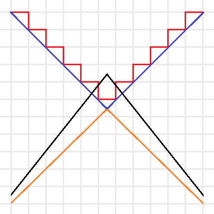
Intuitive sketch of the optimization problems for \(C(f)\) (Red), \(Adv^*(f)\) (Blue), \(Adv(f)\) (Orange), and \(Adv^\pm(f)\) (Black). Note that the red and blue lines are the boundaries of minimization problems, thus their feasible regions are above the boundaries, and the orange and black lines are the boundaries of maximization problems, thus their feasible regions are below the boundaries.

We can simplify this idea with the above picture. The certificate complexity involved a minimization over the integers, so its feasible region is above the boundary drawn by the red line. The optimization problem for \(C(f)\) tries to find the lowest point in the feasible region. The adversary method replaces the integer constraint by real values, and is represented by the blue line. Since the optimization of \(Adv^*(f)\) is still a minimization, this allows us to find lower points in the bigger feasible region. Since the goal of the method is to provide a lower bound, we instead look at \(Adv(f)\) as a maximization problem (with boundary in orange), now the feasible region is below the orange line and any feasible point provides a lower bound. Note that by duality this lower bound is always less than or equal to a feasible point in \(Adv^*(f)\)’s region and thus less than or equal to the certificate complexity. The negative adversary method’s feasible region is represented by the black line. It takes the maximization in \(Adv(f)\) and removes the non-negativity constraint, expanding the feasible region and thus making it possible to find points with \(Adv^\pm(f) > Adv(f)\). Finding natural problems where we have a separation though, has proved to be difficult. In particular, for important problems beyond the certificate complexity barrier (like the collision problem) our best lower bounds come from the polynomial method, and no one has found an approach that uses the negative adversary method directly. Do you know a natural \(f\) such that \(Adv^\pm(f) > Adv(f)\) or better yet, such that \(Adv^\pm(f) > C(f)\)?

Query complexity and the negative adversary method

Of course, without context the method is not very useful. It is the fact that it lower bounds quantum query complexity that first made it a useful tool. Given a function \(f: D \subseteq \{0,1\}^n \rightarrow \{0,1\}\), we have:

\[ Q_\epsilon(f) \geq \frac{1 – 2\sqrt{\epsilon(1 – \epsilon)}}{2} Adv^{\pm}(f) \]

To prove this relation, we think of an adversary holding a quantum superposition \(|\delta\rangle\) over oracle strings instead of the oracle representing a specific input. This \(|\delta\rangle\) is found by the negative adversary method, and corresponds to any eigenvalue of \(\Gamma\) with eigenvalue \(||\Gamma||\). Thus, any algorithm for solving the problem starts with the initial state (refer to the query complexity post for background on notation):

\[ |\Psi_0\rangle = \delta_x |x\rangle_I \otimes |1,0\rangle_Q |0\rangle_W \]

We then consider the reduced density matrix \(\rho_t = Tr_I |\Psi_t\rangle\langle \Psi_t |\) that the adversary holds. This state begins with no entanglement, and in order to learn \(x\) we must create a lot of entanglement in the state. Specifically, we define a progress function \(W^t = \langle \Gamma, \rho_t \rangle\) and show 3 points:

1. \(W^0 = ||\Gamma||\).
2. \(W^t – W^{t+1} \leq 2 \max_j ||\Gamma \cdot \sum_{x,y:x_j \neq y_j} |x\rangle\langle y | ||\)
3. \(W^T = 2\sqrt{\epsilon(1 – \epsilon}||\Gamma||\)

The first step is obvious from our choice of the adversary’s initial state and progress function. The second step is an application of Cauchy–Schwarz and triangle inequalities. The third-step demands that the algorithm give the correct output: \(||\Pi_{f(x)} |\psi_x^T\rangle ||^2 \geq 1 – \epsilon\). This is the most difficult step, and the proof goes through a few special choices of operators and an application of Holder’s inequality. We reference the reader to the original paper [HLS07] for details.

Where do we go from here?

Does the negative adversary method answer if some questions are harder than others? Next time we will see that by looking at span program we can show that the negative adversary method characterizes query complexity: \(Q(f) = \Theta(Adv^\pm(f))\). Thus, the method is a great way to show that some questions are more difficult than others. It also behaves well with respect to iterated functions. In particular, to break the certificate complexity barrier, we can iterate the Kushilevitz-Ambainus partial function \(f\) on 6 bits, defined as:

• Zero inputs of \(f\) are: \( 111000, 011100, 001110, 100110, 110010, 101001, 010101, 001011, 100101, 010011\),
• One inputs of \(f\) are: \( 000111, 100011, 110001, 011001, 001101, 010110, 101010, 110100, 011010, 101100\).

We leave it as an exercise to the eager reader to use their favorite SDP solver to show that \( Adv^\pm(f) \geq 2 + 3\sqrt{5}/5 > C(f) = 3\).

References

[Amb00] A. Ambainis. Quantum lower bounds by quantum arguments. In Proceedings of the thirty-second annual ACM symposium on Theory of computing, pages 636-643. ACM, 2000, arXiv:quant-ph/0002066v1.

[Amb03] A. Ambainis. Polynomial degree vs. quantum query complexity. In Foundations of Computer Science, 2003. Proceedings. 44th Annual IEEE Symposium on, pages 230{239. IEEE, 2003, arXiv:quant-ph/0305028.

[BSS03] H. Barnum, M. Saks, and M. Szegedy. Quantum decision trees and semidefinite programming. In Proc. of 18th IEEE Complexity, pages 179-193, 2003.

[HLS07] Peter Hoyer, Troy Lee, and Robert Spalek. Negative weights make adversaries stronger. 2007, arXiv:quant-ph/0611054v2.

[HNS02] P. Hoyer, J. Neerbek, and Y. Shi. Quantum complexities of ordered searching, sorting, and element distinctness. Algorithmica, 34(4):429-448, 2002, arXiv:quant-ph/0102078.

[LM04] S. Laplante and F. Magniez. Lower bounds for randomized and quantum query complexity using Kolmogorov arguments. 2004, arXiv:quant-ph/0311189.

[Rei09] Ben W. Reichardt. Span programs and quantum query complexity: The general adversary bound is nearly tight for every boolean function. In 2009 50th Annual IEEE Symposium on Foundations of Computer Science, pages 544-551. IEEE, 2009, arXiv:0904.2759v1 [quant-ph].

[Rei11] Ben W. Reichardt. Quantum query complexity. Tutorial at QIP2011 Singapore, 2011.

[SS06] Robert Spalek and Mario Szegedy. All quantum adversary methods are equivalent. Theory of Computing, 2:1-18, 2006, arXiv:quant-ph/0409116v3.

[Zha05] S. Zhang. On the power of Ambainis lower bounds. Theoretical Computer Science, 339(2-3):241-256, 2005, arXiv:quant-ph/0311060.

A folk theorem is a mathematical fact that is generally known (at least by experts), even though its proof may never have appeared in print, or may be difficult to locate.  Recently, cstheory user Eli asked for a citation to a proof of the following folk theorem.

If $latex G$ is a graph with maximum degree 3 and is a minor of $latex H$, then $latex G$ is a topological minor of $latex H$.

Wikipedia mentions this to be true, and refers to Reinhard Diestel’s excellent book on graph theory.  Diestel’s book asserts its truth as well, but does not give a proof.

Graph $latex G$ is a minor of graph $latex H$, if $latex G$ can be obtained from $latex H$ by removing edges in $latex H$ and identifying the vertices that were previously the endpoints of the now-deleted edge.  So, in a sense, we can say that $latex H$ “has local structures that looks like” $latex G$ if $latex G$ is a minor of $latex H$.  It is sometimes possible to prove strong properties about the global structure of $latex H$ if we are guaranteed that $latex H$ has no minors of a certain type, because then no local area of $latex H$ can look a certain way, so it is possible to say something about the entire graph.  The most famous example of this is Wagner’s Theorem, which states that a graph is planar iff neither $latex K_5$ nor $latex K_{3,3}$ is a minor of it.

A topological minor is a related notion.  Informally, $latex G$ is a topological minor of $latex H$ if we can start with $latex G$, and transform it into a subgraph of $latex H$ by only adding vertices into edges that already exist (i.e., subdividing edges, so edge $latex (u,v)$ becomes two edges, $latex (u,x)$ and $latex (x,v)$).  Figure 1 on this web page shows examples of a minor and a topological minor.  (Note: that figure may be behind a paywall.  If anyone knows a good diagram explaining minor vs. topological minor that is freely available, please put it in the comments.)

Fortunately for Eli, Robin Kothari and co-authors had needed this folk theorem for a paper, and they had been unable to find a proof of it either, so they reproved it themselves.  Kothari’s proof (and answer to Eli’s question) appears here.  It is an example of a growing number of original proofs that appear on cstheory.  That proof by Kothari is definitely my “favorite answer of the week.”  As Eli put it, “This is stellar.”