Are some questions harder than others?

Last time we quantified hardness of answering a question with a quantum computer as the quantum query complexity. We promised that this model would allow us to develop techniques for proving lower bounds. In fact, in this model there are two popular tools: the polynomial method, and the (negative) adversary method.

The original version of the quantum adversary method, was proposed by Ambainis [Amb00]. The method starts by choosing two sets of inputs on which \(f\) takes different values. Then the lower bound is determined by combinatorial properties of the graph of the chosen inputs. Some functions, such as sorting or ordered search, could not be satisfactorily lower-bounded by the unweighted adversary method. Hoyer, Neerbek, and Shi [HNS02] weighted the input pairs and obtained the lower bound by evaluating the spectral norm of the Hilbert matrix. Barnum, Saks, and Szegedy [BSS03] proposed a complex general method and described a special case, the spectral method, which gives a lower bound in terms of spectral norms of an adversary matrix. Ambainis also published a weighted version of his adversary method [Amb03]. He showed that it is stronger than the unweighted method but this method is slightly harder to apply, because it requires one to design a weight scheme, which is a quantum counterpart of the classical hard distribution on inputs. Zhang [Zha05] observed that Ambainis had generalized his oldest method in two independent ways, so he united them, and published a strong weighted adversary method. Finally, Laplante and Magniez [LM04] used Kolmogorov complexity in an unusual way and described a Kolmogorov complexity method. Spalek and Szegedy [SS06] unified the above methods into one equivalent method that can be formulated as a semidefinite program (SDP).

We will present an alternative development observed by Reichardt in terms of optimization problems [Rei11]. Our approach will use SDP duality extensively, but we will not prove the duals explicitly, referring the interested reader to previous literature instead [SS06, Rei09].

From certificate complexity to the adversary method

The certificate complexity of a function \(f\) is the non-deterministic version of query complexity and can be found by solving the following optimization problem:

\[ \begin{aligned} C(f) & = \min_{\vec{p}_x \in \{0,1\}^n} \max_x ||\vec{p}_x||^2 \\ \text{s.t.} & \sum_{j:x_j \neq y_j} p_x[j]p_y[j] \geq 1 \quad \text{if} \; f(x) \neq f(y) \end{aligned} \]

We think of \(\vec{p}_x\) as a bit-vector with the \(j\)-th component telling us if index \(j\) is in the certificate or not. The constraint is simply the contrapositive of the definition of certificate complexity: if \(f(x) \neq f(y)\) then there must be at least one bit of overlap on the certificates of \(x\) and \(y\) such that they differ on that bit. The discrete nature of the bit-vector makes certificate complexity a difficult optimization, and it is natural to consider a relaxation:

\[ \begin{aligned} Adv^*(f) & = \min_{\vec{p}_x \in \mathbb{R}^n} \max_x ||\vec{p}_x||^2 \\ \text{s.t.} & \sum_{j:x_j \neq y_j} p_x[j]p_y[j] \geq 1 \quad \text{if} \; f(x) \neq f(y) \end{aligned} \]

Note the suggestive name: the above equation corresponds to the dual of the adversary method. Its more common form is the primal version:

\[ \begin{aligned} Adv(f) & = \max_{\Gamma \in \mathbb{R}^{|D| \times |D|}} ||\Gamma|| \\ \text{s.t.} & \forall j \quad ||\Gamma \cdot \sum_{x,y:x_j \neq y_j} |x\rangle\langle y | || \leq 1 \\ & \Gamma[x,y] = 0 \quad \text{if} \; f(x) = f(y) \\ & \Gamma[x,y] \geq 0 \end{aligned} \]

Since the adversary bound is a relaxation of the certificate complexity, we know that \(Adv(f) \leq C(f)\) for all \(f\). In fact, two even stronger barrier stands in the way of the adversary method: the certificate and property testing barriers. The certificate barrier is that for all functions \(f\), \(Adv(f) \leq \min { \sqrt{C_0(f)n}, \sqrt{C_1(f)n} }\), and if \(f\) is total, then we have \(Adv(f) \leq \sqrt{C_0(f) C_1(f)}\) [Zha05, SS06]. The property testing barrier is for partial functions, where every zero-input is of Hamming distance at least \(\epsilon n\) from every one-input. In that case the method does not yield a lower bound better than \(1/\epsilon\).

Negative adversary method

To overcome these barriers, Hoyer, Lee, and Spalek [HLS07] introduced the negative adversary method. The method is a relaxation of the adversary method that allows negative weights in the adversary matrix:

\[ \begin{aligned} Adv^{\pm}(f) & = \max_{\Gamma \in \mathbb{R}^{|D| \times |D|}} ||\Gamma|| \\ \text{s.t.} & \forall j \quad ||\Gamma \cdot \sum_{x,y:x_j \neq y_j} |x\rangle\langle y | || \leq 1 \\ & \Gamma[x,y] = 0 \quad \text{if} \; f(x) = f(y) \end{aligned} \]

Note that we started with certificate complexity and relaxed that to get the dual of the adversary method. We took the dual to get the adversary method, and then relaxed the adversary method to get the negative adversary method. Since we relaxed in both directions in two different ways, the negative adversary method is not clearly related to the certificate complexity.

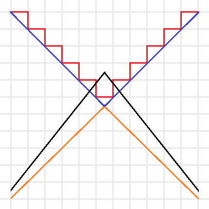
Intuitive sketch of the optimization problems for \(C(f)\) (Red), \(Adv^*(f)\) (Blue), \(Adv(f)\) (Orange), and \(Adv^\pm(f)\) (Black). Note that the red and blue lines are the boundaries of minimization problems, thus their feasible regions are above the boundaries, and the orange and black lines are the boundaries of maximization problems, thus their feasible regions are below the boundaries.

We can simplify this idea with the above picture. The certificate complexity involved a minimization over the integers, so its feasible region is above the boundary drawn by the red line. The optimization problem for \(C(f)\) tries to find the lowest point in the feasible region. The adversary method replaces the integer constraint by real values, and is represented by the blue line. Since the optimization of \(Adv^*(f)\) is still a minimization, this allows us to find lower points in the bigger feasible region. Since the goal of the method is to provide a lower bound, we instead look at \(Adv(f)\) as a maximization problem (with boundary in orange), now the feasible region is below the orange line and any feasible point provides a lower bound. Note that by duality this lower bound is always less than or equal to a feasible point in \(Adv^*(f)\)’s region and thus less than or equal to the certificate complexity. The negative adversary method’s feasible region is represented by the black line. It takes the maximization in \(Adv(f)\) and removes the non-negativity constraint, expanding the feasible region and thus making it possible to find points with \(Adv^\pm(f) > Adv(f)\). Finding natural problems where we have a separation though, has proved to be difficult. In particular, for important problems beyond the certificate complexity barrier (like the collision problem) our best lower bounds come from the polynomial method, and no one has found an approach that uses the negative adversary method directly. Do you know a natural \(f\) such that \(Adv^\pm(f) > Adv(f)\) or better yet, such that \(Adv^\pm(f) > C(f)\)?

Query complexity and the negative adversary method

Of course, without context the method is not very useful. It is the fact that it lower bounds quantum query complexity that first made it a useful tool. Given a function \(f: D \subseteq \{0,1\}^n \rightarrow \{0,1\}\), we have:

\[ Q_\epsilon(f) \geq \frac{1 – 2\sqrt{\epsilon(1 – \epsilon)}}{2} Adv^{\pm}(f) \]

To prove this relation, we think of an adversary holding a quantum superposition \(|\delta\rangle\) over oracle strings instead of the oracle representing a specific input. This \(|\delta\rangle\) is found by the negative adversary method, and corresponds to any eigenvalue of \(\Gamma\) with eigenvalue \(||\Gamma||\). Thus, any algorithm for solving the problem starts with the initial state (refer to the query complexity post for background on notation):

\[ |\Psi_0\rangle = \delta_x |x\rangle_I \otimes |1,0\rangle_Q |0\rangle_W \]

We then consider the reduced density matrix \(\rho_t = Tr_I |\Psi_t\rangle\langle \Psi_t |\) that the adversary holds. This state begins with no entanglement, and in order to learn \(x\) we must create a lot of entanglement in the state. Specifically, we define a progress function \(W^t = \langle \Gamma, \rho_t \rangle\) and show 3 points:

1. \(W^0 = ||\Gamma||\).
2. \(W^t – W^{t+1} \leq 2 \max_j ||\Gamma \cdot \sum_{x,y:x_j \neq y_j} |x\rangle\langle y | ||\)
3. \(W^T = 2\sqrt{\epsilon(1 – \epsilon}||\Gamma||\)

The first step is obvious from our choice of the adversary’s initial state and progress function. The second step is an application of Cauchy–Schwarz and triangle inequalities. The third-step demands that the algorithm give the correct output: \(||\Pi_{f(x)} |\psi_x^T\rangle ||^2 \geq 1 – \epsilon\). This is the most difficult step, and the proof goes through a few special choices of operators and an application of Holder’s inequality. We reference the reader to the original paper [HLS07] for details.

Where do we go from here?

Does the negative adversary method answer if some questions are harder than others? Next time we will see that by looking at span program we can show that the negative adversary method characterizes query complexity: \(Q(f) = \Theta(Adv^\pm(f))\). Thus, the method is a great way to show that some questions are more difficult than others. It also behaves well with respect to iterated functions. In particular, to break the certificate complexity barrier, we can iterate the Kushilevitz-Ambainus partial function \(f\) on 6 bits, defined as:

• Zero inputs of \(f\) are: \( 111000, 011100, 001110, 100110, 110010, 101001, 010101, 001011, 100101, 010011\),
• One inputs of \(f\) are: \( 000111, 100011, 110001, 011001, 001101, 010110, 101010, 110100, 011010, 101100\).

We leave it as an exercise to the eager reader to use their favorite SDP solver to show that \( Adv^\pm(f) \geq 2 + 3\sqrt{5}/5 > C(f) = 3\).

References

[Amb00] A. Ambainis. Quantum lower bounds by quantum arguments. In Proceedings of the thirty-second annual ACM symposium on Theory of computing, pages 636-643. ACM, 2000, arXiv:quant-ph/0002066v1.

[Amb03] A. Ambainis. Polynomial degree vs. quantum query complexity. In Foundations of Computer Science, 2003. Proceedings. 44th Annual IEEE Symposium on, pages 230{239. IEEE, 2003, arXiv:quant-ph/0305028.

[BSS03] H. Barnum, M. Saks, and M. Szegedy. Quantum decision trees and semidefinite programming. In Proc. of 18th IEEE Complexity, pages 179-193, 2003.

[HLS07] Peter Hoyer, Troy Lee, and Robert Spalek. Negative weights make adversaries stronger. 2007, arXiv:quant-ph/0611054v2.

[HNS02] P. Hoyer, J. Neerbek, and Y. Shi. Quantum complexities of ordered searching, sorting, and element distinctness. Algorithmica, 34(4):429-448, 2002, arXiv:quant-ph/0102078.

[LM04] S. Laplante and F. Magniez. Lower bounds for randomized and quantum query complexity using Kolmogorov arguments. 2004, arXiv:quant-ph/0311189.

[Rei09] Ben W. Reichardt. Span programs and quantum query complexity: The general adversary bound is nearly tight for every boolean function. In 2009 50th Annual IEEE Symposium on Foundations of Computer Science, pages 544-551. IEEE, 2009, arXiv:0904.2759v1 [quant-ph].

[Rei11] Ben W. Reichardt. Quantum query complexity. Tutorial at QIP2011 Singapore, 2011.

[SS06] Robert Spalek and Mario Szegedy. All quantum adversary methods are equivalent. Theory of Computing, 2:1-18, 2006, arXiv:quant-ph/0409116v3.

[Zha05] S. Zhang. On the power of Ambainis lower bounds. Theoretical Computer Science, 339(2-3):241-256, 2005, arXiv:quant-ph/0311060.

How hard is it to answer a question? As theoretical computer scientists, this query haunts us. We formalize a ‘question’ as a function on some input and ‘answering’ as running a finite procedure. This procedure might run on a Turing Machine, your cellphone, or a quantum computer. ‘Hard’ is quantified by use of resources such as energy, space or time. Unfortunately, the most popular notion of hardness — time complexity — is notoriously difficult to characterize in a quantum computing model. If we want to show what a model of computation can and can’t do, we must use a related, but simpler measure of complexity. For quantum computing this measure is quantum query complexity. This post explains quantum query complexity and lays the foundations for future entries that will introduce the lower bound technique of the (negative) adversary method, and show how it characterizes quantum query complexity through its connection to span programs.

In the query model, the input to our algorithm is given as a black-box (called the oracle). We can only gain knowledge about the input by asking the oracle for individual bits. The input is a bit-string \( x \in D \subseteq \{0, 1\}^n \) and the goal is to compute some function \(f : D \rightarrow \{0,1\}\). If \(D = \{0,1\}^n\) then we call the function total. For simplicity, we only consider decision problems (binary range), although the machinery has been developed for functions over finite strings in arbitrary finite input and output alphabets.

The query complexity of a function is the minimum number of queries used by any circuit computing the function. For a two-sided error \(\epsilon\), we denote the query complexity by \(Q_\epsilon(f)\). Since success amplification is straightforward, we abbreviate further by setting \(Q(f) = Q_{1/3}(f)\). Similar measures exist for classical algorithms, where this model is more frequently referred to as decision-tree complexity. The usual notation is \(D(f)\) for deterministic query complexity, \(R(f)\) for two-sided error (\(1/3\)) randomized query complexity, and \(C(f)\) for certificate (or non-deterministic) complexity. We specify our model concretely, following [HS05]:

Quantum query model: formally

The memory of a quantum query algorithm is described by three Hilbert spaces (registers): the input register, \(H_I\), which holds the input \(x \in D\), the query register, \(H_Q\), which holds an integer \(1 \leq i \leq n\) and a bit \(b \in \{0,1\}\), and the working memory, \(H_W\), which holds an arbitrary value. The query register and working memory together form the memory accessible to the algorithm, denoted \(H_A\). The unitaries that define the algorithm can only act on this space. The accessible memory of a quantum query algorithm is initialized to a fixed state. On input \(x\) the initial state of the algorithm is \(|x\rangle_I \otimes |1, 0\rangle_Q \otimes |0\rangle_W\). The state of the algorithm then evolves through queries, which depend on the input register, and accessible memory operators which do not.

A query is a unitary operator where the oracle answer is given in the phase. We definite the operator \(O\) by its action on the basis state \(|x\rangle_I \otimes |i,b\rangle_Q\) as

\[ O |x\rangle_I \otimes |i,b\rangle_Q = (-1)^{bx_i} |x\rangle_I \otimes |i,b\rangle_Q \]

The accessible memory operator is an arbitrary unitary operation \(U\) on the accessible memory \(H_A\). This operation is extended to act on the whole space by interpreting it as \(I_I \otimes U\) and \(O\) is interpreted as \(O \otimes I_W\). Thus the state of the algorithm on input \(x\) after \(t\) queries can be written as:

\[ |x\rangle_I |\psi^t_x\rangle_A = U_t O U_{t-1} … U_1 O U_0 |x\rangle_I |1, 0\rangle_Q |0\rangle_W \]

Where we noticed that the input register is left unchanged by the algorithm. The output of a \(T\)-query algorithm is distributed according to the state of the accessible memory \(|\psi^T_x\rangle\) and two projections \(\Pi_0\) and \(\Pi_1\) such that \(\Pi_0 + \Pi_1 = I\) corresponding to the possible outcomes of a decision problem. The probability that given input \(x\) the algorithm returns \(0\) is \(||\Pi_0|\psi^T_x\rangle||^2\) and \(1\) is \(||\Pi_1|\psi^T_x\rangle||^2\). \(Q_\epsilon(f)\) is the minimum number of queries made by an algorithm which outputs \(f(x)\) with probability \(1 – \epsilon\) for every \(x\).

Relations between models

For partial functions, the quantum query complexity can be exponentially smaller than randomized or deterministic query complexity [Sho95, BV97, Sim97, Aar10]. However, if the partial function is invariant under permuting inputs and outputs then the complexities are polynomially related with \(R(f) = O(Q(f)^9)\) [AA09]. If the function is total, then \(D(f)\) is bounded by \(O(Q(f)^6)\) , \(O(Q(f)^4)\) for monotone total functions, and \(O(Q(f)^2)\) for symmetric total functions [BBC+01]. However, no greater than quadratic separations are known for total functions (this separation is achieved by \(OR\), for example). This has led to the conjecture that for total functions \(D(f) = O(Q(f)^2)\). This conjecture is open for all classes of total functions, except monotone [BBC+01], read-once [BS04], and constant-sized 1-certificate functions.

The infamous time complexity is always at least as large as the query complexity since each query takes one unit step. For famous algorithms such as Grover’s search [Gro96] and Shor’s period finding (which is the quantum part of his famed polynomial time factoring algorithm) [Sho95], the time complexity is within poly-logarithmic factors of the query complexity. There are also exceptions to the tight correspondence. The Hidden Subgroup Problem has polynomial query complexity [EHK04], yet polynomial time algorithms are not known for the problem.

By taking the computation between queries as free, we get a handle for producing lower bounds. This allows us to develop strong information-theoretic techniques for lower bounding quantum query complexity. In my next post I will use this framework to develop the (negative) adversary method.

References

[AA09] Scott Aaronson and Andris Ambainis. The need for structure in quantum speedups. 2009, arXiv:0911.0996v1 [quant-ph].

[Aar10] Scott Aaronson. BQP and the polynomial hierarchy. In Proceedings of the 42nd ACM symposium on Theory of computing, pages 141-150. ACM, 2010, arXiv:0910.4698 [quant-ph].

[BBC+01] R. Beals, H. Buhrman, R. Cleve, M. Mosca, and R. de Wolf. Quantum lower bounds by polynomials. Journal of the ACM (JACM), 48(4):778-797, 2001.

[BS04] H. Barnum, and M. Saks. A lower bound on the quantum query complexity of read-once functions. Journal of Computer and System Sciences, 69(2):244-258, 2004. arXiv:quant-ph/0201007v1

[BV97] E. Bernstein and U. Vazirani. Quantum complexity theory. SIAM J. Comput., 26(5):1411-1473, 1997.

[EHK04] M. Ettinger, P. Hoyer, and E. Knill. The quantum query complexity of the hidden subgroup problem is polynomial. Information Processing Letters, 91(1):43-48, 2004, arXiv:quant-ph/0401083v1.

[Gro96] L.K. Grover. A fast quantum mechanical algorithm for database search. In Proceedings of the twenty-eighth annual ACM symposium on Theory of computing, pages 212-219. ACM, 1996, arXiv:quant-ph/9605043.

[HS05] P. Hoyer, and R. Spalek. Lower Bounds on Quantum Query Complexity. Bulletin of the European Association for Theoretical Computer Science, 87, 2005. arXiv:quant-ph/0509153v1.

[Sim97] D.R. Simon. On the power of quantum computation. SIAM Journal on Computing, 26:1474, 1997.

[Sho95] P.W. Shor. Polynomial-time algorithms for prime factorization and discrete logarithms on a quantum computer. SIAM J. Comput., 26:1484-1509, 1995, arXiv:quant-ph/9508027.