This is the second of a two-part series on quantifier elimination over the reals. In the first part, we introduced the Tarski-Seidenberg quantifier elimination theorem. The goal of this post is to give a direct and completely elementary proof of this result.

Before embarking on the proof journey, there’s something we can immediately note. It’s enough to prove quantifier elimination for formulas of the following type:

$latex \displaystyle \phi(y_1,\dots,y_m) = \exists x \bigwedge_{i=1}^n \left( p_i(x,y_1,y_2,\dots, y_m)~\Sigma_i~ 0\right)&fg=000000$

where each $latex {\Sigma_i \in \{<,=,>\}}&fg=000000$ and each $latex {p_i \in {\mathbb R}[x][y_1, \dots, y_m]}&fg=000000$ is a polynomial over the reals. Why? Well, if one quantifier can be eliminated, then we can inductively eliminate all of them. And we can always convert the single quantifier to an $latex {\exists}&fg=000000$ by negation if necessary and then distribute the $latex {\exists}&fg=000000$ over disjunctions to arrive at a boolean combination of formulas of the type above.

I will try to describe now how we could “rediscover” a quantifier elimination procedure due to Albert Muchnik. My description is based on a very nice exposition by Michaux and Ozturk but with some shortcuts and a more staged revealing of the full details. The specific algorithm for quantifier elimination we describe will be much less efficient than the current state-of-the-art described in the previous post. The focus here is on clarity of presentation instead of performance.

We will complete the proof in three stages.

1. $latex {m = 0}&fg=000000$ and linear polynomials

First, let’s restrict ourselves to the simplest case: $latex {m = 0}&fg=000000$ and all the polynomials $latex {p_i}&fg=000000$ are of degree one. In fact, let’s even start with a specific example:

$latex \displaystyle \phi = \exists x ((x+1 > 0) \wedge (-2x+3>0) \wedge (x > 0))&fg=000000$

We will partition the real line into a constant number of intervals so that none of the functions changes sign inside any of the intervals. If we do this, then to decide $latex {\phi}&fg=000000$, we merely have to examine the finitely many intervals to see if on any of them, the three functions ($latex {x+1, -2x+3}&fg=000000$, and $latex {x}&fg=000000$) are all positive.

Each of the linear functions has one root and is always negative on one side of the root and always positive on the other. We will keep ourselves from using the exact value of the root, even though finding it here is trivial, because this will help us in the general case. Whether the function is negative to the left or right side of the root depends on the sign of the leading coefficient. So, the first function $latex {x+1}&fg=000000$ has a root at $latex {\gamma_1}&fg=000000$, is always negative to the left of $latex {\gamma_1}&fg=000000$ and always positive to the left.

The second function, $latex {-2x+3}&fg=000000$, has another root $latex {\gamma_2}&fg=000000$, is always negative to its right, and always positive to its left. How do we know if $latex {\gamma_2}&fg=000000$ is to the left or right of $latex {\gamma_1}&fg=000000$? Well, $latex {-2x+3 = -2(x+1) + 5}&fg=000000$, and since $latex {\gamma_1}&fg=000000$ is a root of $latex {x+1}&fg=000000$, it follows that $latex {-2\gamma_1 + 3 = 5 > 0}&fg=000000$. So, $latex {\gamma_1}&fg=000000$ is to the left of $latex {\gamma_2}&fg=000000$. This results in the following sign configuration diagram (for each pair of signs, the first indicates the sign of $latex {x+1}&fg=000000$, the second the sign of $latex {-2x+3}&fg=000000$):

Finally, the third function $latex {x}&fg=000000$ has a root $latex {\gamma_3}&fg=000000$, is always negative to the left, and always positive to the right. Also, $latex {x = (x+1)-1}&fg=000000$ and $latex {x=-\frac{1}{2}(-2x+3) + 1.5}&fg=000000$, and so $latex {x}&fg=000000$ is negative at $latex {\gamma_1}&fg=000000$ and positive at $latex {\gamma_2}&fg=000000$. This means the following sign configuration diagram:

Since there exists an interval $latex {(\gamma_3,\gamma_2)}&fg=000000$ on which the sign configuration is the desired $latex {(+,+,+)}&fg=000000$, it follows that $latex {\phi}&fg=000000$ evaluates to true. The algorithm we described via this example will obviously work for any $latex {\phi}&fg=000000$ with $latex {m=0}&fg=000000$ and linear inequalities.

2. $latex {m=0}&fg=000000$ and general polynomials

Now, let’s see what changes if some of the polynomials are of higher degree with $latex {m}&fg=000000$ still equal to $latex {0}&fg=000000$:

$latex \displaystyle \psi = \exists \left( \bigwedge_{i=1}^n p_i(x) \Sigma_i 0\right)&fg=000000$

where each $latex {\Sigma_i \in \{<,>,=\}}&fg=000000$. Again, we’ll try to find a sign configuration diagram and check at the end if any of the intervals is described by the wanted sign configuration.

If we try to implement this approach, a fundamental issue crops up. Suppose $latex {p_i}&fg=000000$ is a degree $latex {d}&fg=000000$ polynomial and we know that $latex {p_i(\gamma_1) > 0}&fg=000000$ and $latex {p_i(\gamma_2)>0}&fg=000000$. In the case $latex {p_i}&fg=000000$ was linear, we could safely conclude that $latex {p_i(x)}&fg=000000$ is positive everywhere in the interval $latex {(\gamma_1,\gamma_2)}&fg=000000$. Not so fast here! It could very well be for a higher degree polynomial $latex {p_i}&fg=000000$ that it becomes negative somewhere in between $latex {\gamma_1}&fg=000000$ and $latex {\gamma_2}&fg=000000$. But note that this would mean $latex {p_i’ = \frac{\partial}{\partial x} p_i}&fg=000000$ must change sign somewhere at $latex {\gamma_3 \in (\gamma_1, \gamma_2)}&fg=000000$ by Rolle’s theorem. New idea then! Let’s also partition according to the sign changes of $latex {p_i’}&fg=000000$, a degree $latex {(d-1)}&fg=000000$ polynomial. Suppose we have done so successfully by an inductive argument on the degree, and $latex {\gamma_3}&fg=000000$ is the only sign change occurring in $latex {(\gamma_1, \gamma_2)}&fg=000000$ for $latex {p_i’}&fg=000000$.

We now want to also know the sign of $latex {p_i(\gamma_3)}&fg=000000$. Imitating what we did for $latex {d=1}&fg=000000$, note that if $latex {q_i = (p_i \text{ mod } p_i’)}&fg=000000$, then $latex {p_i(\gamma_3) = q_i(\gamma_3)}&fg=000000$ since $latex {\gamma_3}&fg=000000$ is a root of $latex {p_i’}&fg=000000$. The polynomial $latex {q_i}&fg=000000$ is degree less than $latex {d-1}&fg=000000$, so let’s assume by induction that we know the sign pattern of $latex {q_i}&fg=000000$ as well. Thus, we have at hand the sign of $latex {p_i(\gamma_3)}&fg=000000$.

There are now two situations that can happen. First is if $latex {p_i(\gamma_3) > 0}&fg=000000$ or $latex {p_i(\gamma_3) = 0}&fg=000000$.

This is because $latex {p_i}&fg=000000$ reaches the minimum in $latex {(\gamma_1, \gamma_2)}&fg=000000$ at $latex {\gamma_3}&fg=000000$, and since $latex {p_i(\gamma_3) \geq 0}&fg=000000$, $latex {p_i}&fg=000000$ is not negative anywhere in $latex {(\gamma_1, \gamma_2)}&fg=000000$.

The other situation is the case $latex {p_i(\gamma_3)<0}&fg=000000$. By the intermediate value theorem, $latex {p_i}&fg=000000$ has a root $latex {\gamma_4}&fg=000000$ in $latex {(\gamma_1,\gamma_3)}&fg=000000$ and a root $latex {\gamma_5}&fg=000000$ in $latex {(\gamma_3, \gamma_2)}&fg=000000$.

Note again that because $latex {\gamma_3}&fg=000000$ is the only root of $latex {p_i’}&fg=000000$ in the interval $latex {(\gamma_1, \gamma_2)}&fg=000000$, there cannot be more than one sign change of $latex {p_i}&fg=000000$ between $latex {\gamma_1}&fg=000000$ and $latex {\gamma_3}&fg=000000$ and between $latex {\gamma_3}&fg=000000$ and $latex {\gamma_2}&fg=000000$.

So, from these considerations, it’s clear that knowing the signs of the derivatives of the functions $latex {p_i}&fg=000000$ and of the remainders with respect to these derivatives is very helpful. But of course, obtaining these signs might recursively entail working with the second derivatives and so forth. Thus, let’s define the following hierarchy of collections of polynomials:

$latex \displaystyle \mathcal{P}_0 = \{p_1, \dots, p_n\}&fg=000000$

$latex \displaystyle \mathcal{P}_1 = \mathcal{P}_0 \cup \{p’ : p \in \mathcal{P}_0\} \cup \{(p \text{ mod } q) : p,q \in \mathcal{P}_0, \deg(p)\geq \deg(q)\}&fg=000000$

$latex \displaystyle \dots&fg=000000$

$latex \displaystyle \mathcal{P}_{i} = \mathcal{P}_{i-1} \cup \{p’ : p \in \mathcal{P}_{i-1}\} \cup \{(p \text{ mod } q) : p,q \in \mathcal{P}_{i-1}, \deg(p)\geq \deg(q)\}&fg=000000$

$latex \displaystyle \dots&fg=000000$

The degree of the new polynomials added decreases at each stage. So, there is some $latex {k}&fg=000000$ such that $latex {\mathcal{P}_k}&fg=000000$ doesn’t grow anymore. Let $latex {\mathcal{P}_k = \{t_1, t_2, \dots, t_N\}}&fg=000000$ with $latex {\deg(t_1) \leq \deg(t_2) \leq \cdots \leq \deg(t_N)}&fg=000000$. Note that $latex {N}&fg=000000$ is bounded as a function of $latex {n}&fg=000000$ (though the bound is admittedly pretty poor).

Now, we construct the sign configuration diagram for the polynomials $latex {\{t_1, t_2, \dots, t_N\}}&fg=000000$, starting from that of $latex {t_1}&fg=000000$ (a constant), then adding $latex {t_2}&fg=000000$, and so on. When adding $latex {t_i}&fg=000000$, the real line has already been partitioned according to the roots of $latex {t_1, \dots, t_{i-1}}&fg=000000$. As described earlier, $latex {\text{sign}(t_i)}&fg=000000$ at a root $latex {\gamma}&fg=000000$ of $latex {t_j}&fg=000000$ is the sign of $latex {(t_i \text{ mod } t_j)}&fg=000000$ at $latex {\gamma}&fg=000000$, which has already been computed inductively. Then, we can proceed according to the earlier discussion by partitioning into two any interval where there’s a change in the sign of $latex {t_i}&fg=000000$. The only other technicality is that the sign of $latex {t_i}&fg=000000$ at $latex {-\infty}&fg=000000$ and its sign at $latex {+\infty}&fg=000000$ are not determined by the other polynomials. But these are easy to find given the parity of the degree of $latex {t_i}&fg=000000$ and the sign of its leading coefficient.

3. $latex {m>0}&fg=000000$ and general polynomials

Finally, consider the most general case, $latex {m>0}&fg=000000$ and arbitrary bounded degree polynomials. Let’s interpret $latex {{\mathbb R}[x,y_1,y_2,\dots, y_m]}&fg=000000$ as polynomials in $latex {x}&fg=000000$ with coefficients that are polynomials in $latex {y_1, \dots, y_m}&fg=000000$, and try to push through what we did above. We can start by extending the definitions of the hierarchy of collections of polynomials. Suppose $latex {p(x,\mathbf{y}) = p_D(\mathbf{y}) x^D + p_{D-1}(\mathbf{y}) x^{D-1} + \cdots + p_0(\mathbf{y})}&fg=000000$ and $latex {q(x,\mathbf{y}) = q_E(\mathbf{y}) x^E + q_{E-1}(\mathbf{y}) x^{E-1} + \cdots + q_0(\mathbf{y})}&fg=000000$ with $latex {d \leq D}&fg=000000$ the largest integer such that $latex {p_d(\mathbf{y}) \neq 0}&fg=000000$, $latex {e \leq E}&fg=000000$ the largest integer such that $latex {q_e(\mathbf{y}) \neq 0}&fg=000000$, and $latex {d \geq e}&fg=000000$. One problem is that $latex {(p \text{ mod } q)}&fg=000000$, as a polynomial in $latex {x}&fg=000000$, may not have polynomials in $latex {y}&fg=000000$ as its coefficients. To skirt this issue, let:

$latex \displaystyle (p\text{ zmod } q) = q_e(\mathbf{y}) p(x,\mathbf{y}) – p_d(\mathbf{y})x^{d-e} q(x,\mathbf{y})&fg=000000$

Then, whenever $latex {q(x,\mathbf{y}) = 0}&fg=000000$, the sign of $latex {p(x,\mathbf{y})}&fg=000000$ equals the sign of $latex {(p\text{ zmod } q)}&fg=000000$ at $latex {(x,\mathbf{y})}&fg=000000$ divided by the sign of $latex {q_e(\mathbf{y})}&fg=000000$. Moreover, $latex {(p \text{ zmod } q)}&fg=000000$ is a degree $latex {(d-1)}&fg=000000$ polynomial. So, we will want to replace mod by zmod when constructing the collections $latex {\mathcal{P}_i}&fg=000000$. All this is fine except that we have no idea what $latex {d}&fg=000000$ and $latex {e}&fg=000000$ are and what specifically the sign of $latex {q_e(\mathbf{y})}&fg=000000$ is. Recall that $latex {\mathbf{y}}&fg=000000$ is an unknown parameter! So, what to do? Well, the most naive thing: for each polynomial $latex {p}&fg=000000$, let’s just guess whether each coefficient of $latex {p}&fg=000000$ is positive, negative, or zero.

Now, we can define the hierarchy of collections of polynomials $latex {\mathcal{P}_0, \mathcal{P}_1, \dots}&fg=000000$ in the same way as in the previous section, except that here, the polynomials are in $latex {{\mathbb R}[x,y_1, \dots, y_m]}&fg=000000$, we use zmod instead of mod, and each time we add a polynomial, we make a guess about the signs of its coefficients. The degree of the newly added polynomials decreases at each stage, so that there’s some finite bound $latex {k}&fg=000000$ such that $latex {\mathcal{P}_k}&fg=000000$ doesn’t grow anymore. We can now run the procedure described in the previous section to find the sign configuration diagram for $latex {\mathcal{P}_k}&fg=000000$. In the course of this procedure, whenever we need to know the sign of the leading coefficient of a polynomial, we use the value already guessed for it. Finally, we check whether any interval in the sign configuration diagram contains the desired sign pattern.

Consider the whole set of guesses we’ve made in the course of arriving at this sign configuration diagram. Notice that the total number of guesses is finite, bounded as a function of $latex {n}&fg=000000$. Now, let’s call the set of guesses good if it results in a sign configuration diagram that indeed contains an interval with the wanted sign pattern. Our final quantifier-free formula is a disjunction over all good sets of guesses that checks whether the given input values of $latex {y_1, \dots, y_m}&fg=000000$ is consistent with a good set of guesses.

by Arnab Bhattacharyya

About a month ago, Ankur Moitra dropped by my office. We started chatting about what each of us was up to. He told me a story about a machine learning problem that he was working on with Sanjeev Arora, Rong Ge, and Ravi Kannan. On its face, it was not even clear that the problem (non-negative rank) was decidable, let alone solvable in polynomial time. But on the other hand, they observed that previous work had already shown the existence of an algorithm using quantifier elimination. Ankur was a little taken aback by the claim, by the power of quantifier elimination. He knew of the theory somewhere in the back of his mind, in the same way that you probably know of Brownian motion or universal algebra (possible future topics in this “Something you should know about” series!), but he’d never had the occasion to really use it till then. On the train ride back home, he realized that quantifier elimination not only showed decidability of the problem but could also be helpful in devising a more efficient algorithm.

Quantifier elimination has a bit of a magical feel to it. After the conversation with Ankur, I spent some time revisiting the area, and this post is a consequence of that. I’ll mainly focus on the theory over the reals. It’s a remarkable result that you definitely should know about!

1. What is Quantifier Elimination?

A zeroth-order logic deals with declarative propositions that evaluate to either true or false. It is defined by a set of symbols, a set of logical operators, some inference rules and some axioms. A first-order logic adds functions, relations and quantifiers to the mix. Some examples of sentences in a first-order logic:

$latex \displaystyle \forall x~ \exists y~(y = x^2)&fg=000000$

$latex \displaystyle \forall y~ \exists x~(y = x^2)&fg=000000$

$latex \displaystyle \forall x,y~((x+y)^2 > 4xy \wedge x-y>0)&fg=000000$

The above are examples of sentences, meaning that they contain no free variables (i.e., variables that are not bounded by the quantifiers), whereas a formula $latex {\phi(x_1,\dots,x_n)}&fg=000000$ has $latex {x_1, \dots, x_n}&fg=000000$ as free variables. A quantifier-free formula is one in which no variable in the formula is quantified. Thus, note that a quantifier-free sentence is simply a proposition.

Definition 1 A first-order logic is said to admit quantifier elimination if for any formula $latex {\phi(x_1,\dots,x_n)}&fg=000000$, there exists a quantifier-free formula $latex {\psi(x_1,\dots,x_n)}&fg=000000$ which is logically equivalent to $latex {\phi(x_1,\dots,x_n)}&fg=000000$.

If the quantifier elimination process can be described algorithmically, then decidability of sentences in the logic reduces to decidability of quantifier-free sentences which is often a much easier question. (Note though that algorithmic quantifier elimination of formulas is a stronger condition than decidability of sentences.)

2. Quantifier Elimination over the Reals

The real numbers, being an infinite system, cannot be exactly axiomatized using first-order logic because of the Löwenheim-Skolem Theorem. But the axioms of ordered fields along with the intermediate value theorem yields a natural first-order logic, called the real closed field. The real closed field has the same first-order properties as the reals.

Tarski (1951) showed that the real closed field admits quantifier elimination. As a consequence, one has the following (Seidenberg was responsible for popularizing Tarski’s result):

Theorem 2 (Tarski-Seidenberg) Suppose a formula $latex {\phi(y_1,\dots,y_m)}&fg=000000$ over the real closed field is of the following form: \begin{equation*} Q_1x_1~Q_2x_2~\cdots Q_nx_n~(\rho(y_1,\dots,y_m,x_1,\dots,x_n)) \end{equation*} where $latex {Q_i \in \{\exists,\forall\}}&fg=000000$ and $latex {\rho}&fg=000000$ is a boolean combination of equalities and inequalities of the form:

$latex \displaystyle f_i(y_1,\dots,y_m,x_1,\dots,x_n) = 0&fg=000000$

$latex \displaystyle g_i(y_1,\dots,y_m,x_1,\dots,x_n) > 0&fg=000000$

where each $latex {f_i}&fg=000000$ and $latex {g_i}&fg=000000$ is a polynomial with coefficients in $latex {{\mathbb R}}&fg=000000$, mapping $latex {{\mathbb R}^{m+n}}&fg=000000$ to $latex {{\mathbb R}}&fg=000000$. Then, one can explicitly construct a logically equivalent formula $latex {\phi'(y_1, \dots, y_m)}&fg=000000$ of the same form but quantifier-free. Moreover, there is a proof of the equivalence that uses only the axioms of ordered fields and the intermediate value theorem for polynomials.

I should be more explicit about what “explicitly construct” means. Usually, it is assumed that the coefficients of the polynomials $latex {f_i}&fg=000000$ and $latex {g_i}&fg=000000$ are integers, so that there is a bound on the complexity of the quantifier elimination algorithm in terms of the size of the largest coefficient. (If the coefficients are integers, all the computations only involve integers.) But, even when the coefficients are real numbers, there is a bound on the “arithmetic complexity” of the algorithm, meaning the number of arithmetic operations $latex {+, -, \times, \div}&fg=000000$ performed with infinite precision.

A quick example. Suppose we are given an $latex {r}&fg=000000$-by-$latex {s}&fg=000000$ matrix $latex {M = (M_{i,j})}&fg=000000$, and we’d like to find out whether the rows of $latex {M}&fg=000000$ are linearly dependent, i.e. the following condition:

$latex \displaystyle \exists \lambda_1, \dots, \lambda_r \left( \neg \left(\bigwedge_{i=1}^r (\lambda_i = 0)\right) \wedge \bigwedge_{j=1}^s (\lambda_1 M_{1,j}+\lambda_2 M_{2,j} + \cdots \lambda_m M_{r,j} = 0) \right)&fg=000000$

Tarski-Seidenberg immediately asserts an algorithm to transform the above formula into one that does not involve the $latex {\lambda_i}&fg=000000$’s, only the entries of the matrix. Of course, for this particular example, we have an extremely efficient algorithm (Gaussian elimination) but quantifier elimination gives a much more generic explanation for the decidability of the problem.

2.1. Semialgebraic sets

If $latex {m=0}&fg=000000$ in Theorem 2, then Tarski-Seidenberg produces a proposition with no variables that can then be evaluated directly, such as in the linear dependency example. This shows that the feasibility of semialgebraic setsis a decidable problem. A semialgebraic set $latex {S}&fg=000000$ is a finite union of sets of the form:

$latex \displaystyle \{x \in {\mathbb R}^n~|~f_i(x) = 0, g_j(x) > 0 \text{ for all }i=1,\dots, \ell_1, j= 1,\dots, \ell_2\}&fg=000000$

where $latex {f_1,\dots, f_{\ell_1}, g_1,\dots, g_{\ell_2}: {\mathbb R}^n \rightarrow {\mathbb R}}&fg=000000$ are $latex {n}&fg=000000$-variate polynomials over the reals. The feasibility problem for a semialgebraic set $latex {S}&fg=000000$ is deciding if $latex {S}&fg=000000$ is empty or not. An algorithm to decide feasibility directly follows from applying quantifier elimination.

Note that this is in stark contrast to the first-order theory over the integers for which Godel’s Incompleteness Theorem shows undecidability. Also, over the rationals, Robinson proved undecidability (in her Ph.D. thesis advised by Tarski) by showing how to express any first-order sentence over the integers as a first-order sentence over the rationals. This latter step now has several different proofs. Poonen has written a nice survey of (un)decidability of first-order theories over various domains.

2.2. Efficiency

What about the complexity of quantifier elimination over the reals? The algorithm proposed by Tarski does not even show complexity that is elementary recursive! The situation was much improved by Collins (1975) who gave a doubly-exponential algorithm using a technique called “cylindrical algebraic decomposition”. More precisely, the running time of the algorithm is $latex {poly(C,(\ell d)^{2^{O(n)}})}&fg=000000$, where $latex {C}&fg=000000$ measures the size of the largest coefficient in the polynomials, $latex {\ell}&fg=000000$ is the number of polynomials, $latex {d}&fg=000000$ is the maximum degree of the polynomials, and $latex {n}&fg=000000$ is the total number of variables.

A more detailed understanding of the complexity of quantifier elimination emerged from an important work of Ben-Or, Kozen and Reif (1986). Their main contribution was an ingenious polynomial time algorithm to test the consistency of univariate polynomial constraints: given a set of univariate polynomials $latex {{f_i}}&fg=000000$ and a system of constraints of the form $latex {f_i(x) \leq 0}&fg=000000$, $latex {f_i(x) = 0}&fg=000000$ or $latex {f_i(x) > 0}&fg=000000$, does the system have a solution $latex {x}&fg=000000$? Such an algorithm exists despite the fact that it’s not known how to efficiently find an $latex {x}&fg=000000$ that makes the signs of the polynomials attain a given configuration. Ben-Or, Kozen and Reif also claimed an extension of their method to multivariate polynomials, but this analysis was later found to be flawed.

Nevertheless, subsequent works have found clever ways to reduce to the univariate case. These more recent papers have shown that one can make the complexity of the quantification elimination algorithm be only singly exponential if the number of quantifier alternations (number of switches between $latex {\exists}&fg=000000$ and $latex {\forall}&fg=000000$) is bounded or if the model of computation is parallel. See Basu (1999) for the current record and for references to prior work.

As for lower bounds, Davenport and Heintz (1988) showed that doubly-exponential time is required for quantifier elimination, by explicitly constructing formulas for which the length of the quantifier-free expression blows up doubly-exponentially. Brown and Davenport (2007) showed that the doubly exponential dependence is necessary even when all the polynomials in the first order formula are linear and there is only one free variable. I do not know if a doubly exponential lower bound is known for the decision problem when there are no free variables.

Thanks to Ankur for helpful suggestions. Part II of this post will contain a relatively quick proof of Tarski’s theorem! Stay tuned.

Alfred Tarski (1951). A Decision Method for Elementary Algebra and Geometry Rand Corporation

I saw a nice result sketched a few weeks ago, on the “online matching” problem. Below I try to re-explain the result, using some idiomatic (and as a bonus, inoffensive) terminology which I find makes it easier to remember what’s going on.

Online Matching. There is a set of items, call them Lunches, which you want to get eaten. There is a set of people who will arrive in a sequence, call them Diners. Each Diner is willing to eat certain Lunches but not others. Once a Diner shows up, you can give them any remaining Lunch they like, but that Lunch cannot be re-sold again. The prototypical problem is that a Diner might show up but you already sold all of the Lunches that they like. Your task: find a (randomized) strategy to maximize the (expected) number of Lunches sold, relative to the maximum Lunch-Diner matching size.

This is an online problem: you don’t have all the information about Diner preferences before the algorithm begins, and you need to start committing to decisions before you know everyone’s preferences in full.

Consider the following strategy:

Algorithm: pick a random ordering/permutation of the lunches; then when a diner arrives, give her the first available lunch in the ordering that she likes.

How does this perform? In expectation at least (1-1/e)M lunches are sold, where M is the maximum (offline) matching size in the Lunch-Diner graph. But proving so is tricky. (This ratio 1-1/e turns out to be the best possible.) Birnbaum and Mathieu recently gave a simpler proof that this ratio is achieved. Amin Saberi, whose talk sketched this, rightly pointed out that it feels like a “proof from The Book!”

With a small lemma (e.g. Lemma 2 in Birnbaum-Mathieu), we may assume that the number of diners and lunches are equal, and that there is a perfect matching between diners and lunches. Let the number of diners and lunches each be n, and so M=n.

Let x_t be the probability that in a random lunch permutation, upon running Algorithm, the lunch in position t is eaten.

Experiment 1. Take a random lunch permutation. Score 1 if the lunch at position t is not eaten, 0 if it is eaten. The expected value of this experiment is 1-x_t.

Experiment 2. Take a random lunch permutation, and a random diner. Score 1 if that diner eats a lunch in one of the first t positions, 0 otherwise. The expected value of this experiment is (x₁ + … + x_t)/n.

The key is to show that the second experiment has expected value greater than or equal to the first one, then we will finish up by an easy calculation. We do this with a joint experiment, similar to “coupling” arguments.

Joint experiment. Let t be fixed. Take a random lunch permutation π₁, and look at the lunch L in position t. Let D be matched to L in the perfect matching. Obtain π₂ from π₁ by removing L and re-inserting L in a random position.

Key claim: π₂ and D are independent, uniformly distributed random variables. This implies that we can run both experiments at the same time using this joint distribution on π₁, π₂, L, D. Moreover,

Deterministic Lemma. For any π₁, and for an uneaten lunch L at position t in π₁, obtain π₂ from π₁ by removing L and re-inserting L in any position. Let D be matched to L in the perfect matching. Then in π₂, D eats one of the first t lunches.

This implies that whenever experiment 1 scores a point, so does experiment 2. So taking expectations,

(x₁ + … + x_t)/n ≥ 1-x_t.

This equation is the crux. Let x_≤t = x₁+…+x_t, then we see x_≤t ≥ (ⁿ/_n+1)(1+x_≤t-1). This recursion is easy to unravel and it gives a lower bound of n(1-(ⁿ/_n+1)ⁿ) ≥ n(1-1/e) on x_≤n, the expected size of the matching!

(This is a cross-post from my blog, which has posts commonly on math and/or lunches.)

In our first post on learning theory, we’ll start by examining a nice question that started an interesting discussion and brought out some of the core issues learning theorists constantly have to deal with.  It also serves as a good introduction to one of the classic areas of learning theory.

The Question

Laszlo Kozma asked the following question:  Is finding the minimum regular expression an NP complete problem?  Moreover, Laszlo wanted to know if this has any connections to learning regular languages.  This question and the answers to it brought out many subtile points, including issues of representation, consistency, and complexity.

As we know, regular expressions describe regular languages, which are also equivalent to the class of Finite State Automata (DFA), a classic object in computability theory.  Suppose we get examples of strings that are members of a regular language (positive examples) and strings that are not members of the language (negative examples), labeled accordingly.  Laszlo wanted to know whether finding the smallest regular expression (or DFA) consistent with these examples is NP-hard, and moreover, what this has to do with learning regular languages.

Learning and Occam’s Razor

When we talk about learning, we need to first pick a model, and the first natural one to think about is Leslie Valiant’s classical PAC learning model (’84), partly for which he received this year’s Turing award.  In PAC learning, the learner is trying to learn some concept (in this case, a specific regular language) and is given positive and negative examples (member strings and not) from some unknown distribution (say, uniform over all strings). The learner’s goal is to produce a hypothesis that will match the label of the hidden target (the membership in the target regular language) on most examples from the same distribution, with high probability.  The learner has to succeed for every choice of target and every distribution over examples.

Say the learner knows the target class (in our case, that the target is some regular language).  In that case, if the learner gets some polynomially many examples in the representation of the concept and can find a small hypothesis from the target class that is correct on all the examples, even if this hypothesis isn’t exactly equal to the target, it will generalize well and be suitable for PAC learning.  This theorem is aptly named Occam’s Razor (Blumer et al. ’87).

Hardness of Learning

So, indeed, Laszlo was right — whether or not finding the smallest regular expression (or smallest DFA) consistent with a given set of examples is NP-hard has a lot to do with being able to learn regular languages efficiently.  Note that if we’re not concerned with efficiency, exhaustive search through all automata would yield the smallest one.  But unfortunately, it is indeed NP-hard to find the smallest DFA (Angluin ’78; Gold ’78), and moreover, it is NP-hard to approximate a target DFA of size OPT by a DFA of size OPT^k for any constant factor k (Pitt and Warmuth ’93).

So does this imply regular languages are hard to learn? Unfortunately not; efficiently finding a small, zero error, DFA would have given us an efficient learning algorithm, but just because we can’t find one doesn’t mean there isn’t some other way to learn regular languages.  For example, perhaps, we could learn by finding a hypothesis that’s something else entirely, and not a DFA. (For those interested, this is the difference between proper and improper learning.)  Just because we’ve eliminated one way of learning doesn’t mean we’ve eliminated other venues.

There is, however, a more serious impediment to learning regular languages.  In an important paper, Kearns and Valiant (’94) proved that you can encode the RSA function into a DFA. So, even if the labeled examples come from the uniform distribution, being able to generalize to future examples (also even coming from the uniform distribution) would break the RSA cryptosystem (Rivest et al. ’78), which is quite unlikely. This type of result is known as a cryptographic hardness of learning result. Hence, there is good reason to believe that DFA aren’t efficiently PAC learnable after all.

A Small Puzzle

This question raised a lot of interesting discussion among the answers and in the comments, with the pointers to the crpytographic hardness results bringing up a puzzle.  It is known that given an automaton, there exist algorithms to minimize it efficiently (Huffman ’54; Moore ’56), meaning it is possible to efficiently find the automaton with the smallest number of states that accepts exactly the same language as the given one.  At first, it may seem that contradicts the the NP-hardness result, that one can find the smallest automaton consistent with a given set of examples using the following procedure: construct a large DFA so that for each positive example, we have a chain accepting only that example.  Then, minimize that DFA.  It seems like this should work, but why doesn’t it?

The answer turns out to be that when you construct a DFA using the procedure above, you commit to a certain language.  Then, upon minimizing the DFA, you have to stay within the same language, whereas the smallest DFA consistent with all the examples might encode a different language altogether.  One can easily see this by the following example: imagine the only positive examples are “000001” and “000011.”  Building the DFA in the manner described above commits to the language {“000001”, “000011”}, whereas the smallest DFA consistent with all examples is just one accept state pointing to itself, and that accepts everything (because we have no negative examples, this is allowed).  Puzzle resolved.

Other Models

The question didn’t specify what it means to learn, and one great thing about the cstheory site is that  different answers were able to address learnability in different models.  We’ve just discussed the PAC model and learning regular languages in it, but the picture changes when we consider other models of learning. One model addressed in the answers is Mark Gold’s learning in the limit (’67), the first learning model considered in the literature.  Here, the learner is presented an infinite stream of data and must eventually converge to the correct hypothesis.  It turns out that in this setting, regular languages are unconditionally not learnable in the limit (Gold ’67) from text (positive examples).

To give a positive result, regular language learning is the canonical problem for another model, learning with membership and equivalence queries. In this model, the learner gets to ask membership queries (“Is string [x] in the language?”) and equivalence queries (“Is my hypothesis correct, and if not, what is a string on which it disagrees with the target?”).  In a seminal paper, Dana Angluin (’87), who introduced the model, showed that regular languages are exactly learnable with membership and equivalence queries, and this result helped illustrate the power and relevance of this query model.

Open Problems

Because this is a blog post and not a survey, many important results have been left out from this discussion.  Nonetheless, it may seem that everything is already known about the learnability of automata. This is far from true.  There are many interesting problems left to explore: What happens for specific subclasses of reglar languages? Can we learn when the target language isn’t worst-case, but comes from some distribution? What if we restrict to certain types of algorithms? etc.

But instead of listing many specific questions, we will instead turn to a fascinating (and difficult) question asked on this site which has implications for learning regular languages.  Aryeh Kontorovich recently asked: How many DFAs accept two given strings?  Or, rather, how hard is it to compute this quantity, as a function of n, the number of states in the DFA.  At the time of this post, this question has no accepted answers, so if you think you have an answer, come to cstheory.stackexchange.com and let us know!

References

D. Angluin. On the complexity of minimum inference of regular sets. Information and Control, 3(39):337–350, 1978.

D. Angluin. Learning regaular sets from queries and counterexamples. Information and Computation, 75:87–106, 1987.

A. Blumer, A. Ehrenfeucht, D. Haussler, M. K. Warmuth. Occam’s razor. Information Processing Letters 24, 377-380, 1987.

E. M. Gold. Language identification in the limit. Information and Control, 10:447–474, 1967.

E. M. Gold. Complexity of automaton identification from given data. Information and Control, 3(37):302–420, 1978.

D. A. Huffman: The Synthesis of Sequential Switching Circuits. Journal of the Franklin Institute 257: 161-190 34, 1954.

E. F. Moore: Gedanken-experiments on sequential machines. Automata Studies. Princeton University Press, 129-15, 1956.

L. Pitt and M. Warmuth. The minimum consistent DFA problem cannot be approximated within any polynomial. Journal of the Association for Computing Machinery, 40(1):95–142, 1993.

R. L. Rivest, A. Shamir, and L. Adleman. A method for obtaining digital signatures and public-key cryptosystems. Communications of the ACM, Volume 21 Issue 2, Feb. 1978.

L. G.  Valiant. A Theory of the Learnable. Communications of the ACM, 1984,

Are some questions harder than others?

Last time we quantified hardness of answering a question with a quantum computer as the quantum query complexity. We promised that this model would allow us to develop techniques for proving lower bounds. In fact, in this model there are two popular tools: the polynomial method, and the (negative) adversary method.

The original version of the quantum adversary method, was proposed by Ambainis [Amb00]. The method starts by choosing two sets of inputs on which \(f\) takes different values. Then the lower bound is determined by combinatorial properties of the graph of the chosen inputs. Some functions, such as sorting or ordered search, could not be satisfactorily lower-bounded by the unweighted adversary method. Hoyer, Neerbek, and Shi [HNS02] weighted the input pairs and obtained the lower bound by evaluating the spectral norm of the Hilbert matrix. Barnum, Saks, and Szegedy [BSS03] proposed a complex general method and described a special case, the spectral method, which gives a lower bound in terms of spectral norms of an adversary matrix. Ambainis also published a weighted version of his adversary method [Amb03]. He showed that it is stronger than the unweighted method but this method is slightly harder to apply, because it requires one to design a weight scheme, which is a quantum counterpart of the classical hard distribution on inputs. Zhang [Zha05] observed that Ambainis had generalized his oldest method in two independent ways, so he united them, and published a strong weighted adversary method. Finally, Laplante and Magniez [LM04] used Kolmogorov complexity in an unusual way and described a Kolmogorov complexity method. Spalek and Szegedy [SS06] unified the above methods into one equivalent method that can be formulated as a semidefinite program (SDP).

We will present an alternative development observed by Reichardt in terms of optimization problems [Rei11]. Our approach will use SDP duality extensively, but we will not prove the duals explicitly, referring the interested reader to previous literature instead [SS06, Rei09].

From certificate complexity to the adversary method

The certificate complexity of a function \(f\) is the non-deterministic version of query complexity and can be found by solving the following optimization problem:

\[ \begin{aligned} C(f) & = \min_{\vec{p}_x \in \{0,1\}^n} \max_x ||\vec{p}_x||^2 \\ \text{s.t.} & \sum_{j:x_j \neq y_j} p_x[j]p_y[j] \geq 1 \quad \text{if} \; f(x) \neq f(y) \end{aligned} \]

We think of \(\vec{p}_x\) as a bit-vector with the \(j\)-th component telling us if index \(j\) is in the certificate or not. The constraint is simply the contrapositive of the definition of certificate complexity: if \(f(x) \neq f(y)\) then there must be at least one bit of overlap on the certificates of \(x\) and \(y\) such that they differ on that bit. The discrete nature of the bit-vector makes certificate complexity a difficult optimization, and it is natural to consider a relaxation:

\[ \begin{aligned} Adv^*(f) & = \min_{\vec{p}_x \in \mathbb{R}^n} \max_x ||\vec{p}_x||^2 \\ \text{s.t.} & \sum_{j:x_j \neq y_j} p_x[j]p_y[j] \geq 1 \quad \text{if} \; f(x) \neq f(y) \end{aligned} \]

Note the suggestive name: the above equation corresponds to the dual of the adversary method. Its more common form is the primal version:

\[ \begin{aligned} Adv(f) & = \max_{\Gamma \in \mathbb{R}^{|D| \times |D|}} ||\Gamma|| \\ \text{s.t.} & \forall j \quad ||\Gamma \cdot \sum_{x,y:x_j \neq y_j} |x\rangle\langle y | || \leq 1 \\ & \Gamma[x,y] = 0 \quad \text{if} \; f(x) = f(y) \\ & \Gamma[x,y] \geq 0 \end{aligned} \]

Since the adversary bound is a relaxation of the certificate complexity, we know that \(Adv(f) \leq C(f)\) for all \(f\). In fact, two even stronger barrier stands in the way of the adversary method: the certificate and property testing barriers. The certificate barrier is that for all functions \(f\), \(Adv(f) \leq \min { \sqrt{C_0(f)n}, \sqrt{C_1(f)n} }\), and if \(f\) is total, then we have \(Adv(f) \leq \sqrt{C_0(f) C_1(f)}\) [Zha05, SS06]. The property testing barrier is for partial functions, where every zero-input is of Hamming distance at least \(\epsilon n\) from every one-input. In that case the method does not yield a lower bound better than \(1/\epsilon\).

Negative adversary method

To overcome these barriers, Hoyer, Lee, and Spalek [HLS07] introduced the negative adversary method. The method is a relaxation of the adversary method that allows negative weights in the adversary matrix:

\[ \begin{aligned} Adv^{\pm}(f) & = \max_{\Gamma \in \mathbb{R}^{|D| \times |D|}} ||\Gamma|| \\ \text{s.t.} & \forall j \quad ||\Gamma \cdot \sum_{x,y:x_j \neq y_j} |x\rangle\langle y | || \leq 1 \\ & \Gamma[x,y] = 0 \quad \text{if} \; f(x) = f(y) \end{aligned} \]

Note that we started with certificate complexity and relaxed that to get the dual of the adversary method. We took the dual to get the adversary method, and then relaxed the adversary method to get the negative adversary method. Since we relaxed in both directions in two different ways, the negative adversary method is not clearly related to the certificate complexity.

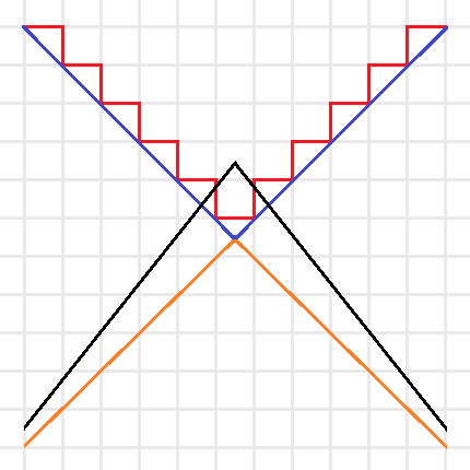
Intuitive sketch of the optimization problems for \(C(f)\) (Red), \(Adv^*(f)\) (Blue), \(Adv(f)\) (Orange), and \(Adv^\pm(f)\) (Black). Note that the red and blue lines are the boundaries of minimization problems, thus their feasible regions are above the boundaries, and the orange and black lines are the boundaries of maximization problems, thus their feasible regions are below the boundaries.

We can simplify this idea with the above picture. The certificate complexity involved a minimization over the integers, so its feasible region is above the boundary drawn by the red line. The optimization problem for \(C(f)\) tries to find the lowest point in the feasible region. The adversary method replaces the integer constraint by real values, and is represented by the blue line. Since the optimization of \(Adv^*(f)\) is still a minimization, this allows us to find lower points in the bigger feasible region. Since the goal of the method is to provide a lower bound, we instead look at \(Adv(f)\) as a maximization problem (with boundary in orange), now the feasible region is below the orange line and any feasible point provides a lower bound. Note that by duality this lower bound is always less than or equal to a feasible point in \(Adv^*(f)\)’s region and thus less than or equal to the certificate complexity. The negative adversary method’s feasible region is represented by the black line. It takes the maximization in \(Adv(f)\) and removes the non-negativity constraint, expanding the feasible region and thus making it possible to find points with \(Adv^\pm(f) > Adv(f)\). Finding natural problems where we have a separation though, has proved to be difficult. In particular, for important problems beyond the certificate complexity barrier (like the collision problem) our best lower bounds come from the polynomial method, and no one has found an approach that uses the negative adversary method directly. Do you know a natural \(f\) such that \(Adv^\pm(f) > Adv(f)\) or better yet, such that \(Adv^\pm(f) > C(f)\)?

Query complexity and the negative adversary method

Of course, without context the method is not very useful. It is the fact that it lower bounds quantum query complexity that first made it a useful tool. Given a function \(f: D \subseteq \{0,1\}^n \rightarrow \{0,1\}\), we have:

\[ Q_\epsilon(f) \geq \frac{1 – 2\sqrt{\epsilon(1 – \epsilon)}}{2} Adv^{\pm}(f) \]

To prove this relation, we think of an adversary holding a quantum superposition \(|\delta\rangle\) over oracle strings instead of the oracle representing a specific input. This \(|\delta\rangle\) is found by the negative adversary method, and corresponds to any eigenvalue of \(\Gamma\) with eigenvalue \(||\Gamma||\). Thus, any algorithm for solving the problem starts with the initial state (refer to the query complexity post for background on notation):

\[ |\Psi_0\rangle = \delta_x |x\rangle_I \otimes |1,0\rangle_Q |0\rangle_W \]

We then consider the reduced density matrix \(\rho_t = Tr_I |\Psi_t\rangle\langle \Psi_t |\) that the adversary holds. This state begins with no entanglement, and in order to learn \(x\) we must create a lot of entanglement in the state. Specifically, we define a progress function \(W^t = \langle \Gamma, \rho_t \rangle\) and show 3 points:

1. \(W^0 = ||\Gamma||\).
2. \(W^t – W^{t+1} \leq 2 \max_j ||\Gamma \cdot \sum_{x,y:x_j \neq y_j} |x\rangle\langle y | ||\)
3. \(W^T = 2\sqrt{\epsilon(1 – \epsilon}||\Gamma||\)

The first step is obvious from our choice of the adversary’s initial state and progress function. The second step is an application of Cauchy–Schwarz and triangle inequalities. The third-step demands that the algorithm give the correct output: \(||\Pi_{f(x)} |\psi_x^T\rangle ||^2 \geq 1 – \epsilon\). This is the most difficult step, and the proof goes through a few special choices of operators and an application of Holder’s inequality. We reference the reader to the original paper [HLS07] for details.

Where do we go from here?

Does the negative adversary method answer if some questions are harder than others? Next time we will see that by looking at span program we can show that the negative adversary method characterizes query complexity: \(Q(f) = \Theta(Adv^\pm(f))\). Thus, the method is a great way to show that some questions are more difficult than others. It also behaves well with respect to iterated functions. In particular, to break the certificate complexity barrier, we can iterate the Kushilevitz-Ambainus partial function \(f\) on 6 bits, defined as:

• Zero inputs of \(f\) are: \( 111000, 011100, 001110, 100110, 110010, 101001, 010101, 001011, 100101, 010011\),
• One inputs of \(f\) are: \( 000111, 100011, 110001, 011001, 001101, 010110, 101010, 110100, 011010, 101100\).

We leave it as an exercise to the eager reader to use their favorite SDP solver to show that \( Adv^\pm(f) \geq 2 + 3\sqrt{5}/5 > C(f) = 3\).

References

[Amb00] A. Ambainis. Quantum lower bounds by quantum arguments. In Proceedings of the thirty-second annual ACM symposium on Theory of computing, pages 636-643. ACM, 2000, arXiv:quant-ph/0002066v1.

[Amb03] A. Ambainis. Polynomial degree vs. quantum query complexity. In Foundations of Computer Science, 2003. Proceedings. 44th Annual IEEE Symposium on, pages 230{239. IEEE, 2003, arXiv:quant-ph/0305028.

[BSS03] H. Barnum, M. Saks, and M. Szegedy. Quantum decision trees and semidefinite programming. In Proc. of 18th IEEE Complexity, pages 179-193, 2003.

[HLS07] Peter Hoyer, Troy Lee, and Robert Spalek. Negative weights make adversaries stronger. 2007, arXiv:quant-ph/0611054v2.

[HNS02] P. Hoyer, J. Neerbek, and Y. Shi. Quantum complexities of ordered searching, sorting, and element distinctness. Algorithmica, 34(4):429-448, 2002, arXiv:quant-ph/0102078.

[LM04] S. Laplante and F. Magniez. Lower bounds for randomized and quantum query complexity using Kolmogorov arguments. 2004, arXiv:quant-ph/0311189.

[Rei09] Ben W. Reichardt. Span programs and quantum query complexity: The general adversary bound is nearly tight for every boolean function. In 2009 50th Annual IEEE Symposium on Foundations of Computer Science, pages 544-551. IEEE, 2009, arXiv:0904.2759v1 [quant-ph].

[Rei11] Ben W. Reichardt. Quantum query complexity. Tutorial at QIP2011 Singapore, 2011.

[SS06] Robert Spalek and Mario Szegedy. All quantum adversary methods are equivalent. Theory of Computing, 2:1-18, 2006, arXiv:quant-ph/0409116v3.

[Zha05] S. Zhang. On the power of Ambainis lower bounds. Theoretical Computer Science, 339(2-3):241-256, 2005, arXiv:quant-ph/0311060.

How hard is it to answer a question? As theoretical computer scientists, this query haunts us. We formalize a ‘question’ as a function on some input and ‘answering’ as running a finite procedure. This procedure might run on a Turing Machine, your cellphone, or a quantum computer. ‘Hard’ is quantified by use of resources such as energy, space or time. Unfortunately, the most popular notion of hardness — time complexity — is notoriously difficult to characterize in a quantum computing model. If we want to show what a model of computation can and can’t do, we must use a related, but simpler measure of complexity. For quantum computing this measure is quantum query complexity. This post explains quantum query complexity and lays the foundations for future entries that will introduce the lower bound technique of the (negative) adversary method, and show how it characterizes quantum query complexity through its connection to span programs.

In the query model, the input to our algorithm is given as a black-box (called the oracle). We can only gain knowledge about the input by asking the oracle for individual bits. The input is a bit-string \( x \in D \subseteq \{0, 1\}^n \) and the goal is to compute some function \(f : D \rightarrow \{0,1\}\). If \(D = \{0,1\}^n\) then we call the function total. For simplicity, we only consider decision problems (binary range), although the machinery has been developed for functions over finite strings in arbitrary finite input and output alphabets.

The query complexity of a function is the minimum number of queries used by any circuit computing the function. For a two-sided error \(\epsilon\), we denote the query complexity by \(Q_\epsilon(f)\). Since success amplification is straightforward, we abbreviate further by setting \(Q(f) = Q_{1/3}(f)\). Similar measures exist for classical algorithms, where this model is more frequently referred to as decision-tree complexity. The usual notation is \(D(f)\) for deterministic query complexity, \(R(f)\) for two-sided error (\(1/3\)) randomized query complexity, and \(C(f)\) for certificate (or non-deterministic) complexity. We specify our model concretely, following [HS05]:

Quantum query model: formally

The memory of a quantum query algorithm is described by three Hilbert spaces (registers): the input register, \(H_I\), which holds the input \(x \in D\), the query register, \(H_Q\), which holds an integer \(1 \leq i \leq n\) and a bit \(b \in \{0,1\}\), and the working memory, \(H_W\), which holds an arbitrary value. The query register and working memory together form the memory accessible to the algorithm, denoted \(H_A\). The unitaries that define the algorithm can only act on this space. The accessible memory of a quantum query algorithm is initialized to a fixed state. On input \(x\) the initial state of the algorithm is \(|x\rangle_I \otimes |1, 0\rangle_Q \otimes |0\rangle_W\). The state of the algorithm then evolves through queries, which depend on the input register, and accessible memory operators which do not.

A query is a unitary operator where the oracle answer is given in the phase. We definite the operator \(O\) by its action on the basis state \(|x\rangle_I \otimes |i,b\rangle_Q\) as

\[ O |x\rangle_I \otimes |i,b\rangle_Q = (-1)^{bx_i} |x\rangle_I \otimes |i,b\rangle_Q \]

The accessible memory operator is an arbitrary unitary operation \(U\) on the accessible memory \(H_A\). This operation is extended to act on the whole space by interpreting it as \(I_I \otimes U\) and \(O\) is interpreted as \(O \otimes I_W\). Thus the state of the algorithm on input \(x\) after \(t\) queries can be written as:

\[ |x\rangle_I |\psi^t_x\rangle_A = U_t O U_{t-1} … U_1 O U_0 |x\rangle_I |1, 0\rangle_Q |0\rangle_W \]

Where we noticed that the input register is left unchanged by the algorithm. The output of a \(T\)-query algorithm is distributed according to the state of the accessible memory \(|\psi^T_x\rangle\) and two projections \(\Pi_0\) and \(\Pi_1\) such that \(\Pi_0 + \Pi_1 = I\) corresponding to the possible outcomes of a decision problem. The probability that given input \(x\) the algorithm returns \(0\) is \(||\Pi_0|\psi^T_x\rangle||^2\) and \(1\) is \(||\Pi_1|\psi^T_x\rangle||^2\). \(Q_\epsilon(f)\) is the minimum number of queries made by an algorithm which outputs \(f(x)\) with probability \(1 – \epsilon\) for every \(x\).

Relations between models

For partial functions, the quantum query complexity can be exponentially smaller than randomized or deterministic query complexity [Sho95, BV97, Sim97, Aar10]. However, if the partial function is invariant under permuting inputs and outputs then the complexities are polynomially related with \(R(f) = O(Q(f)^9)\) [AA09]. If the function is total, then \(D(f)\) is bounded by \(O(Q(f)^6)\) , \(O(Q(f)^4)\) for monotone total functions, and \(O(Q(f)^2)\) for symmetric total functions [BBC+01]. However, no greater than quadratic separations are known for total functions (this separation is achieved by \(OR\), for example). This has led to the conjecture that for total functions \(D(f) = O(Q(f)^2)\). This conjecture is open for all classes of total functions, except monotone [BBC+01], read-once [BS04], and constant-sized 1-certificate functions.

The infamous time complexity is always at least as large as the query complexity since each query takes one unit step. For famous algorithms such as Grover’s search [Gro96] and Shor’s period finding (which is the quantum part of his famed polynomial time factoring algorithm) [Sho95], the time complexity is within poly-logarithmic factors of the query complexity. There are also exceptions to the tight correspondence. The Hidden Subgroup Problem has polynomial query complexity [EHK04], yet polynomial time algorithms are not known for the problem.

By taking the computation between queries as free, we get a handle for producing lower bounds. This allows us to develop strong information-theoretic techniques for lower bounding quantum query complexity. In my next post I will use this framework to develop the (negative) adversary method.

References

[AA09] Scott Aaronson and Andris Ambainis. The need for structure in quantum speedups. 2009, arXiv:0911.0996v1 [quant-ph].

[Aar10] Scott Aaronson. BQP and the polynomial hierarchy. In Proceedings of the 42nd ACM symposium on Theory of computing, pages 141-150. ACM, 2010, arXiv:0910.4698 [quant-ph].

[BBC+01] R. Beals, H. Buhrman, R. Cleve, M. Mosca, and R. de Wolf. Quantum lower bounds by polynomials. Journal of the ACM (JACM), 48(4):778-797, 2001.

[BS04] H. Barnum, and M. Saks. A lower bound on the quantum query complexity of read-once functions. Journal of Computer and System Sciences, 69(2):244-258, 2004. arXiv:quant-ph/0201007v1

[BV97] E. Bernstein and U. Vazirani. Quantum complexity theory. SIAM J. Comput., 26(5):1411-1473, 1997.

[EHK04] M. Ettinger, P. Hoyer, and E. Knill. The quantum query complexity of the hidden subgroup problem is polynomial. Information Processing Letters, 91(1):43-48, 2004, arXiv:quant-ph/0401083v1.

[Gro96] L.K. Grover. A fast quantum mechanical algorithm for database search. In Proceedings of the twenty-eighth annual ACM symposium on Theory of computing, pages 212-219. ACM, 1996, arXiv:quant-ph/9605043.

[HS05] P. Hoyer, and R. Spalek. Lower Bounds on Quantum Query Complexity. Bulletin of the European Association for Theoretical Computer Science, 87, 2005. arXiv:quant-ph/0509153v1.

[Sim97] D.R. Simon. On the power of quantum computation. SIAM Journal on Computing, 26:1474, 1997.

[Sho95] P.W. Shor. Polynomial-time algorithms for prime factorization and discrete logarithms on a quantum computer. SIAM J. Comput., 26:1484-1509, 1995, arXiv:quant-ph/9508027.