Archive for February, 2012

This is the second of a two-part series on quantifier elimination over the reals. In the first part, we introduced the Tarski-Seidenberg quantifier elimination theorem. The goal of this post is to give a direct and completely elementary proof of this result.

Before embarking on the proof journey, there’s something we can immediately note. It’s enough to prove quantifier elimination for formulas of the following type:

$latex \displaystyle \phi(y_1,\dots,y_m) = \exists x \bigwedge_{i=1}^n \left( p_i(x,y_1,y_2,\dots, y_m)~\Sigma_i~ 0\right)&fg=000000$

where each $latex {\Sigma_i \in \{<,=,>\}}&fg=000000$ and each $latex {p_i \in {\mathbb R}[x][y_1, \dots, y_m]}&fg=000000$ is a polynomial over the reals. Why? Well, if one quantifier can be eliminated, then we can inductively eliminate all of them. And we can always convert the single quantifier to an $latex {\exists}&fg=000000$ by negation if necessary and then distribute the $latex {\exists}&fg=000000$ over disjunctions to arrive at a boolean combination of formulas of the type above.

I will try to describe now how we could “rediscover” a quantifier elimination procedure due to Albert Muchnik. My description is based on a very nice exposition by Michaux and Ozturk but with some shortcuts and a more staged revealing of the full details. The specific algorithm for quantifier elimination we describe will be much less efficient than the current state-of-the-art described in the previous post. The focus here is on clarity of presentation instead of performance.

We will complete the proof in three stages.

1. $latex {m = 0}&fg=000000$ and linear polynomials

First, let’s restrict ourselves to the simplest case: $latex {m = 0}&fg=000000$ and all the polynomials $latex {p_i}&fg=000000$ are of degree one. In fact, let’s even start with a specific example:

$latex \displaystyle \phi = \exists x ((x+1 > 0) \wedge (-2x+3>0) \wedge (x > 0))&fg=000000$

We will partition the real line into a constant number of intervals so that none of the functions changes sign inside any of the intervals. If we do this, then to decide $latex {\phi}&fg=000000$, we merely have to examine the finitely many intervals to see if on any of them, the three functions ($latex {x+1, -2x+3}&fg=000000$, and $latex {x}&fg=000000$) are all positive.

Each of the linear functions has one root and is always negative on one side of the root and always positive on the other. We will keep ourselves from using the exact value of the root, even though finding it here is trivial, because this will help us in the general case. Whether the function is negative to the left or right side of the root depends on the sign of the leading coefficient. So, the first function $latex {x+1}&fg=000000$ has a root at $latex {\gamma_1}&fg=000000$, is always negative to the left of $latex {\gamma_1}&fg=000000$ and always positive to the left.

The second function, $latex {-2x+3}&fg=000000$, has another root $latex {\gamma_2}&fg=000000$, is always negative to its right, and always positive to its left. How do we know if $latex {\gamma_2}&fg=000000$ is to the left or right of $latex {\gamma_1}&fg=000000$? Well, $latex {-2x+3 = -2(x+1) + 5}&fg=000000$, and since $latex {\gamma_1}&fg=000000$ is a root of $latex {x+1}&fg=000000$, it follows that $latex {-2\gamma_1 + 3 = 5 > 0}&fg=000000$. So, $latex {\gamma_1}&fg=000000$ is to the left of $latex {\gamma_2}&fg=000000$. This results in the following sign configuration diagram (for each pair of signs, the first indicates the sign of $latex {x+1}&fg=000000$, the second the sign of $latex {-2x+3}&fg=000000$):

Finally, the third function $latex {x}&fg=000000$ has a root $latex {\gamma_3}&fg=000000$, is always negative to the left, and always positive to the right. Also, $latex {x = (x+1)-1}&fg=000000$ and $latex {x=-\frac{1}{2}(-2x+3) + 1.5}&fg=000000$, and so $latex {x}&fg=000000$ is negative at $latex {\gamma_1}&fg=000000$ and positive at $latex {\gamma_2}&fg=000000$. This means the following sign configuration diagram:

Since there exists an interval $latex {(\gamma_3,\gamma_2)}&fg=000000$ on which the sign configuration is the desired $latex {(+,+,+)}&fg=000000$, it follows that $latex {\phi}&fg=000000$ evaluates to true. The algorithm we described via this example will obviously work for any $latex {\phi}&fg=000000$ with $latex {m=0}&fg=000000$ and linear inequalities.

2. $latex {m=0}&fg=000000$ and general polynomials

Now, let’s see what changes if some of the polynomials are of higher degree with $latex {m}&fg=000000$ still equal to $latex {0}&fg=000000$:

$latex \displaystyle \psi = \exists \left( \bigwedge_{i=1}^n p_i(x) \Sigma_i 0\right)&fg=000000$

where each $latex {\Sigma_i \in \{<,>,=\}}&fg=000000$. Again, we’ll try to find a sign configuration diagram and check at the end if any of the intervals is described by the wanted sign configuration.

If we try to implement this approach, a fundamental issue crops up. Suppose $latex {p_i}&fg=000000$ is a degree $latex {d}&fg=000000$ polynomial and we know that $latex {p_i(\gamma_1) > 0}&fg=000000$ and $latex {p_i(\gamma_2)>0}&fg=000000$. In the case $latex {p_i}&fg=000000$ was linear, we could safely conclude that $latex {p_i(x)}&fg=000000$ is positive everywhere in the interval $latex {(\gamma_1,\gamma_2)}&fg=000000$. Not so fast here! It could very well be for a higher degree polynomial $latex {p_i}&fg=000000$ that it becomes negative somewhere in between $latex {\gamma_1}&fg=000000$ and $latex {\gamma_2}&fg=000000$. But note that this would mean $latex {p_i’ = \frac{\partial}{\partial x} p_i}&fg=000000$ must change sign somewhere at $latex {\gamma_3 \in (\gamma_1, \gamma_2)}&fg=000000$ by Rolle’s theorem. New idea then! Let’s also partition according to the sign changes of $latex {p_i’}&fg=000000$, a degree $latex {(d-1)}&fg=000000$ polynomial. Suppose we have done so successfully by an inductive argument on the degree, and $latex {\gamma_3}&fg=000000$ is the only sign change occurring in $latex {(\gamma_1, \gamma_2)}&fg=000000$ for $latex {p_i’}&fg=000000$.

We now want to also know the sign of $latex {p_i(\gamma_3)}&fg=000000$. Imitating what we did for $latex {d=1}&fg=000000$, note that if $latex {q_i = (p_i \text{ mod } p_i’)}&fg=000000$, then $latex {p_i(\gamma_3) = q_i(\gamma_3)}&fg=000000$ since $latex {\gamma_3}&fg=000000$ is a root of $latex {p_i’}&fg=000000$. The polynomial $latex {q_i}&fg=000000$ is degree less than $latex {d-1}&fg=000000$, so let’s assume by induction that we know the sign pattern of $latex {q_i}&fg=000000$ as well. Thus, we have at hand the sign of $latex {p_i(\gamma_3)}&fg=000000$.

There are now two situations that can happen. First is if $latex {p_i(\gamma_3) > 0}&fg=000000$ or $latex {p_i(\gamma_3) = 0}&fg=000000$.

This is because $latex {p_i}&fg=000000$ reaches the minimum in $latex {(\gamma_1, \gamma_2)}&fg=000000$ at $latex {\gamma_3}&fg=000000$, and since $latex {p_i(\gamma_3) \geq 0}&fg=000000$, $latex {p_i}&fg=000000$ is not negative anywhere in $latex {(\gamma_1, \gamma_2)}&fg=000000$.

The other situation is the case $latex {p_i(\gamma_3)<0}&fg=000000$. By the intermediate value theorem, $latex {p_i}&fg=000000$ has a root $latex {\gamma_4}&fg=000000$ in $latex {(\gamma_1,\gamma_3)}&fg=000000$ and a root $latex {\gamma_5}&fg=000000$ in $latex {(\gamma_3, \gamma_2)}&fg=000000$.

Note again that because $latex {\gamma_3}&fg=000000$ is the only root of $latex {p_i’}&fg=000000$ in the interval $latex {(\gamma_1, \gamma_2)}&fg=000000$, there cannot be more than one sign change of $latex {p_i}&fg=000000$ between $latex {\gamma_1}&fg=000000$ and $latex {\gamma_3}&fg=000000$ and between $latex {\gamma_3}&fg=000000$ and $latex {\gamma_2}&fg=000000$.

So, from these considerations, it’s clear that knowing the signs of the derivatives of the functions $latex {p_i}&fg=000000$ and of the remainders with respect to these derivatives is very helpful. But of course, obtaining these signs might recursively entail working with the second derivatives and so forth. Thus, let’s define the following hierarchy of collections of polynomials:

$latex \displaystyle \mathcal{P}_0 = \{p_1, \dots, p_n\}&fg=000000$

$latex \displaystyle \mathcal{P}_1 = \mathcal{P}_0 \cup \{p’ : p \in \mathcal{P}_0\} \cup \{(p \text{ mod } q) : p,q \in \mathcal{P}_0, \deg(p)\geq \deg(q)\}&fg=000000$

$latex \displaystyle \dots&fg=000000$

$latex \displaystyle \mathcal{P}_{i} = \mathcal{P}_{i-1} \cup \{p’ : p \in \mathcal{P}_{i-1}\} \cup \{(p \text{ mod } q) : p,q \in \mathcal{P}_{i-1}, \deg(p)\geq \deg(q)\}&fg=000000$

$latex \displaystyle \dots&fg=000000$

The degree of the new polynomials added decreases at each stage. So, there is some $latex {k}&fg=000000$ such that $latex {\mathcal{P}_k}&fg=000000$ doesn’t grow anymore. Let $latex {\mathcal{P}_k = \{t_1, t_2, \dots, t_N\}}&fg=000000$ with $latex {\deg(t_1) \leq \deg(t_2) \leq \cdots \leq \deg(t_N)}&fg=000000$. Note that $latex {N}&fg=000000$ is bounded as a function of $latex {n}&fg=000000$ (though the bound is admittedly pretty poor).

Now, we construct the sign configuration diagram for the polynomials $latex {\{t_1, t_2, \dots, t_N\}}&fg=000000$, starting from that of $latex {t_1}&fg=000000$ (a constant), then adding $latex {t_2}&fg=000000$, and so on. When adding $latex {t_i}&fg=000000$, the real line has already been partitioned according to the roots of $latex {t_1, \dots, t_{i-1}}&fg=000000$. As described earlier, $latex {\text{sign}(t_i)}&fg=000000$ at a root $latex {\gamma}&fg=000000$ of $latex {t_j}&fg=000000$ is the sign of $latex {(t_i \text{ mod } t_j)}&fg=000000$ at $latex {\gamma}&fg=000000$, which has already been computed inductively. Then, we can proceed according to the earlier discussion by partitioning into two any interval where there’s a change in the sign of $latex {t_i}&fg=000000$. The only other technicality is that the sign of $latex {t_i}&fg=000000$ at $latex {-\infty}&fg=000000$ and its sign at $latex {+\infty}&fg=000000$ are not determined by the other polynomials. But these are easy to find given the parity of the degree of $latex {t_i}&fg=000000$ and the sign of its leading coefficient.

3. $latex {m>0}&fg=000000$ and general polynomials

Finally, consider the most general case, $latex {m>0}&fg=000000$ and arbitrary bounded degree polynomials. Let’s interpret $latex {{\mathbb R}[x,y_1,y_2,\dots, y_m]}&fg=000000$ as polynomials in $latex {x}&fg=000000$ with coefficients that are polynomials in $latex {y_1, \dots, y_m}&fg=000000$, and try to push through what we did above. We can start by extending the definitions of the hierarchy of collections of polynomials. Suppose $latex {p(x,\mathbf{y}) = p_D(\mathbf{y}) x^D + p_{D-1}(\mathbf{y}) x^{D-1} + \cdots + p_0(\mathbf{y})}&fg=000000$ and $latex {q(x,\mathbf{y}) = q_E(\mathbf{y}) x^E + q_{E-1}(\mathbf{y}) x^{E-1} + \cdots + q_0(\mathbf{y})}&fg=000000$ with $latex {d \leq D}&fg=000000$ the largest integer such that $latex {p_d(\mathbf{y}) \neq 0}&fg=000000$, $latex {e \leq E}&fg=000000$ the largest integer such that $latex {q_e(\mathbf{y}) \neq 0}&fg=000000$, and $latex {d \geq e}&fg=000000$. One problem is that $latex {(p \text{ mod } q)}&fg=000000$, as a polynomial in $latex {x}&fg=000000$, may not have polynomials in $latex {y}&fg=000000$ as its coefficients. To skirt this issue, let:

$latex \displaystyle (p\text{ zmod } q) = q_e(\mathbf{y}) p(x,\mathbf{y}) – p_d(\mathbf{y})x^{d-e} q(x,\mathbf{y})&fg=000000$

Then, whenever $latex {q(x,\mathbf{y}) = 0}&fg=000000$, the sign of $latex {p(x,\mathbf{y})}&fg=000000$ equals the sign of $latex {(p\text{ zmod } q)}&fg=000000$ at $latex {(x,\mathbf{y})}&fg=000000$ divided by the sign of $latex {q_e(\mathbf{y})}&fg=000000$. Moreover, $latex {(p \text{ zmod } q)}&fg=000000$ is a degree $latex {(d-1)}&fg=000000$ polynomial. So, we will want to replace mod by zmod when constructing the collections $latex {\mathcal{P}_i}&fg=000000$. All this is fine except that we have no idea what $latex {d}&fg=000000$ and $latex {e}&fg=000000$ are and what specifically the sign of $latex {q_e(\mathbf{y})}&fg=000000$ is. Recall that $latex {\mathbf{y}}&fg=000000$ is an unknown parameter! So, what to do? Well, the most naive thing: for each polynomial $latex {p}&fg=000000$, let’s just guess whether each coefficient of $latex {p}&fg=000000$ is positive, negative, or zero.

Now, we can define the hierarchy of collections of polynomials $latex {\mathcal{P}_0, \mathcal{P}_1, \dots}&fg=000000$ in the same way as in the previous section, except that here, the polynomials are in $latex {{\mathbb R}[x,y_1, \dots, y_m]}&fg=000000$, we use zmod instead of mod, and each time we add a polynomial, we make a guess about the signs of its coefficients. The degree of the newly added polynomials decreases at each stage, so that there’s some finite bound $latex {k}&fg=000000$ such that $latex {\mathcal{P}_k}&fg=000000$ doesn’t grow anymore. We can now run the procedure described in the previous section to find the sign configuration diagram for $latex {\mathcal{P}_k}&fg=000000$. In the course of this procedure, whenever we need to know the sign of the leading coefficient of a polynomial, we use the value already guessed for it. Finally, we check whether any interval in the sign configuration diagram contains the desired sign pattern.

Consider the whole set of guesses we’ve made in the course of arriving at this sign configuration diagram. Notice that the total number of guesses is finite, bounded as a function of $latex {n}&fg=000000$. Now, let’s call the set of guesses good if it results in a sign configuration diagram that indeed contains an interval with the wanted sign pattern. Our final quantifier-free formula is a disjunction over all good sets of guesses that checks whether the given input values of $latex {y_1, \dots, y_m}&fg=000000$ is consistent with a good set of guesses.

I attended the FSTTCS conference that was held in IIT Bombay last December. The conference saw over 180 participants and had many interesting talks. I will discuss a few of them in this post.

Talks from Breakthroughs in TCS workshop

Madhu Sudan. Multiplicity Codes: Locality with High Efficiency.

Madhu Sudan gave a nice talk based on a recent result by Swastik Kopparty, Shubhangi Saraf and Sergey Yekhanin (STOC 2011). He was excited about the result for two reasons. Firstly, unlike other advances in LDCs where applications of the results are found only in other parts of theory, this result actually could be of great practical interest. “It’s the numbers that are making sense” he said. Secondly, the construction of the code is so elegant that you are surprised by its simplicity.

I’ll try to sketch the main idea below:

Background. Suppose we want to send a k-bit message on a noisy channel. A well-known method is to use an error-correcting code to encode the k-bit message x into an n-bit codeword C(x) and transmit the codeword instead of the message x. The codeword C(x) is such that we can recover the original message x from it even if many bits in C(x) get corrupted. A typical way to recover x would be to run a decoder on the (possibly corrupted) C(x).

Two parameters in this scheme are of interest: the redundancy incurred in constructing the codeword C(x) and the efficiency with which we can decode the message x from the codeword. The complexity of encoding is usually ignored since it is not critical in most applications.

The rate of the code is the ratio of message length to codeword length: k/n. The higher the rate, the lesser the redundancy of the code.

LDCs. But what if one is interested only in knowing just a particular bit of the message x? This is where a Locally Decodable Code (LDC) is useful. LDCs allow the reconstruction of any arbitrary bit x_i by looking only at a small number of randomly chosen positions of the received codeword C(x). The query complexity of the code is the number of bits we need to look at in order to recover a particular bit.

Obviously, we desire to have LDCs with high rate and low query complexity. But until now, for codes with rate>1/2, it was unknown how to construct any non-trivial decoding. For rates lower than 1/2, we could construct a code with rate O(ε^Ω(1/ε)) and query complexity O( k^ε) for 0<ε<1. For example, Reed-Muller codes — which are based on evaluating multivariate polynomials.

Bivariate Reed-Muller codes. We briefly describe how polynomials can be useful in coding. Let F_q denote the finite field of cardinality q. Consider the bivariate polynomials over the field F_q. A bivariate polynomial of degree d has ( {d+1 \choose 2} ) monomials. For example, if d=2 the monomials are x²,xy and y². So any polynomial of degree d can be specified by the coefficients of each of these monomials. The coordinates of the message x can be thought of as coefficients of a polynomial P(x,y) of degree d. So our message is of length ( k={d+1 \choose 2} ). Each coordinate of the message has a value from F_q (we call this an alphabet). The codeword C(x) corresponding to the message x is obtained as follows: The coordinates of the codeword is indexed by elements of ( F_{q}^2 ). So the length of the codeword n=q².

The codeword corresponding to the polynomial P(x,y) is the vector C(P) as given below:

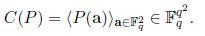
So the first co-ordinate of C(P) would have the value of P(1,1), the second coordinate would have the value of P(1,2), and in general the (i*q+j)th coordinate of C(P) would have the value P(i,j).

The rate of this code is less than 1/2 and it can be shown that the correct value at a particular coordinate of the received codeword can be decoded by making only O(√k) queries on the received codeword, assuming that a constant fraction of the codeword gets corrupted.

Multiplicity codes. The key idea in the paper is to encode the message using multivariate polynomials and their partial derivatives. If we plug this idea to the above example, each coordinate of the codeword will have 3 alphabets instead of one or in other words each coordinate would be a value from ( F_{q}^3 ). So the codeword is now:

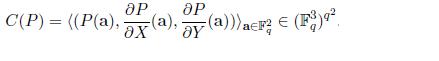
This improves the rate from <1/2 to 2/3! It can be done without increasing the query complexity. This by itself is a new result. What’s more is they can extend this idea to get codes of arbitrarily high rate while keeping the query complexity small. Here is their main theorem from the paper:

For every ε>0, α>0, and for infinitely many k, there exists a code which encodes k-bit messages with rate 1-α, and is locally decodable from some constant fraction of errors using O(k^ε) time and queries.

Umesh Vazirani. Certifiable Quantum Dice.

Background. Many computational tasks such as cryptography, game theoretic protocols, physical simulations, etc. require a source of independent random bits. But constructing a truly random device is a hard task. Even assuming that such a device is available, how do we test if it is working correctly? This task seems impossible since a perfect random number generator must output every n bit sequence with equal probability and there is no reason one can reject a particular output in favor of an other.

Quantum mechanics offers a way to get past this fundamental barrier: starting with O(log² n) random bits one can generate n certifiable random bits.

To get an idea of how this is possible let us consider the CHSH game first (given below).

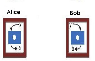The CHSH game. Alice and Bob are two co-operating players who receive inputs x and y, respectively from a third party. Alice and Bob are at two different locations. The winning condition for them is to produce outputs a and b such that the following condition is satisfied: If x=y=1, then a and b must be different. For any of the other three combinations of x and y, the outputs have to be equal. If the players are correlated according to the laws of classical physics, only any three of the four pairs of inputs can be satisfied. So the maximum probability of winning is 0.75. However, if they adopt a strategy based on quantum correlations, this value can be increased to 0.851. See the references in this article in Nature for more details.

We can define a quantum regime corresponding to the success probabilities between 0.75 and 0.85. It is simple to construct two quantum devices corresponding to any value in the regime. But if two devices produce co-relations in the regime, they must be randomized. Or in other words, randomness is for real! This gives a simple statistical test to cerfify randomness.

Result. We are using two random input bits (x,y) to produce two random output bits, so this doesn’t accomplish much. We cannot claim the output to be more random than the input. Vazirani and Vidick in their paper describe a protocol that uses O(log ² n) seed bits to produce n certifiable random bits.

Jaikumar Radhakrishnan. Communication Complexity of Multi-Party Set-Disjointness Problem.

Consider the following problem: Alice and Bob are given inputs x and y respectively and are asked to compute a function f(x,y). They are charged for the number of bits exchanged. The minimum number of bits that have to be exchanged in order to compute the function f is the communication complexity of the problem. A particular problem that is of interest in the area of communication complexity is the set-disjointness problem.

Problem. There are k parties each of whom has a subset from {1,..,n} stuck on his forehead. Each party can see the all the subsets except his own. The set-disjointness problem is to determine if the intersection of all the k subsets is empty. Again, we charge for the number of bits exchanged. All the parties have access to a shared blackboard on which they can write, so we have a broadcast medium.

The case when k=2 is well-understood both in both deterministic and randomized settings. (In randomized version, all the parties have access to a shared source of infinite random bits.)

Results. Until recently, for the general multi-party case, the best lower bound on communication complexity known for the number-on-the-forehead model was Ω(n^1/k+1/2^{k^2}). Last year, Sherstov improved this bound to Ω(n/4^k)^1/4 which is close to tight.

Jaikumar is a fantastic teacher. In what was basically a blackboard-talk, he gave an overview of the main ideas in Sherstov’s proof in a way that was accessible even to non communication-complexity experts. The arguments are based on approximating Boolean functions by polynomials.

Other talks in BTCS

There were several other good talks. Naveen Garg surveyed the recent progress on approximation algorithms for the Traveling Salesman Problem that achieve a strictly better than 1.5 approximation factor. Manindra presented the result on lower bound on ACC by Ryan Williams. Aleksender Madry gave two talks: one in which he presented a new randomized algorithm for the k-server problem that achieves poly-logarithmic competitiveness and one on approximating max-flow in capacitated, undirected graphs using the techniques from electrical flows and laplacian systems. Nisheeth Vishnoi discussed new algorithms for the Unique Games Conjecture. Amit Kumar gave a talk about a recent result by Friedman, Hansen and Zwick on proving lower bounds for randomized pivoting rules in simplex algorithm. Sanjeev Khanna spoke about some recent progress on the approximability of the edge-disjoint paths problem. Most of these results are now famous in theory-circles.

Conference talks

There were 38 papers out of which about 16 were from Theory A. Here are some of the talks I attended:

The Semi-stochastic Ski-rental Problem. (Aleksander Mądry and Debmalya Panigrahi)

An online algorithm is an algorithm which optimizes a given function when the entire input in not known in advance, but is rather revealed sequentially. The algorithm has to make irrevocable choices about the output as the input is seen. The ratio of the performance of the online algorithm to the optimal offline algorithm is called the competitive ratio of the algorithm.

On one hand, we have online models which assume nothing about the input and on the other we have stochastic models which assume that the input comes from a known distribution. The semi-stochastic model in this paper unifies these two extremes. In this model, the algorithm does not know the input distribution initially, but can learn the distribution by asking queries. The algorithm has a certain query budget. If the budget is zero (resp. infinite), the model reduces to the online (resp. stochastic) version. The goal is to maximize the competitive ratio assuming that the queries are answered adversarially.

This model is well-motivated because in many real world situations, the online model is too pessimistic and the stochastic model is too optimistic. We can usually learn the input distribution to some extent and often learning the distribution incurs some cost.

Problem. The ski-rental problem is studied in this framework. The problem is as follows: Ann wants to go skiing, but she does not know the exact number of days she would like to ski. Each morning she has to decide if she has to rent a pair of skis or buy them. Renting the skis cost 1 unit/day and buying them would cost b units. The goal is to minimize the total cost.

Here is a trivial 2-competitive algorithm: Rent the skis for b-1 days. If she decides to go on the bth day, then buy them. This is the best one can do in a deterministic setting. The best randomized algorithm gives a competitive ratio of e/(e-1).

Results. Given a desired competitive ratio e/(e-1)+ε, the paper gives lower and upper bounds on the number of queries that need to be asked in order to achieve that ratio. The lower bound is C/ε (where C is a universal constant) and the upper bound is O(1/ε^1.5).

Rainbow Connectivity: Hardness and Tractability. Prabhanjan Ananth, Meghana Nasre, and Kanthi K Sarpatwar.

Problem. In an edge-colored graph, a rainbow path is a path in which all the edges have different colors. Given a graph G, can we color the edges using k colors such that every pair of vertices has a rainbow path between them? In short, is rc(G) ≤ k? A graph is said to be rainbow connected if the above condition is satisfied. Further, for every pair, if one of the shortest paths between them is a rainbow path, then the graph is said to be strongly rainbow connected (src(G)).

Results.The paper shows that determining if src(G) ≤ k is NP-hard even for bipartite graphs. The hardness of determining if rc(G) ≤ k was open for the case when k is odd. The authors establish the hardness for this case (for every odd k≥3) by an indirect reduction from vertex coloring problem. The argument is combinatorial in nature. I’m not sure if the same argument can be tweaked for the case when k is even (which might simplify the overall proof of hardness for every k≥3.)

Simultaneously Satisfying Linear Equations Over F₂. (by Robert Crowston et. al)

Problem. We are given a set of m equations containing n variables x₁,…,x_n of the form ∏_i∈Ix_i=b. The x_is and b take values from {-1,1}. For example, equations can be x₁x₄x₈=1, x₂x₅x_n=-1, etc. Each equation is associated with a positive weight. The objective is to find an assignment of variables such that the total weight of the satisfied equations is maximized.

The problem is known to be NP-Hard, so we concentrate on a special case. Let the total weight of all the equations be W. If we randomly assign 1 or -1 to each variable, every equation gets satisfied with probability 1/2. Hence, there is always an assignment that is guaranteed to give a weight of W/2. The problem MAX-LIN[k] is to find the complexity of finding an assignment with weight W/2+k, where k is the parameter.

Roughly, a problem is said to be fixed-parameter-tractable (FPT) is if an input instance containing n input bits and an integer k (called the parameter) can be solved in time f(k)n^O(1), where f(k) depends only on the parameter k.

Results. The authors show that the problem MAX-LIN[k] is FPT and admits a kernel of size O(k² log k) and give an O(2^{O(klog k)}(nm)^c) algorithm. They also have new results for a variant of the problem where the number of variables in the equation is fixed to a constant. The results in the paper is built on the previous results by the same authors some parts of which use Fourier analysis of pseudo-Boolean functions. I’m not familiar with these techniques.

Obtaining a Bipartite Graph by Contracting Few Edges. (by Pinar Heggernes et. al)

Problem. Given a graph G, can we obtain a bipartite graph by contracting k edges? This problem though simple to state was not studied before. Which is quite surprising considering that the related problem of removing vertices to obtain a bipartite graph is a central problem in parametrized complexity.

Results. The main result of the paper shows that the problem is fixed-parameter-tractable when parametrized by k. The result makes use of many techniques well-known in parametrized complexity like iterative compression, irrelevant vertex and important separators. An interesting open question is to decide if the problem admits a polynomial kernel.

The update complexity of selection and related problems. (Manoj Gupta, Yogish Sabharwal, and Sandeep Sen)

Problem. We want to compute the function f(x₁,x₂,…,x_n) when the x_is are not known precisely but rather just known to lie in an interval. We are allowed to query and update a particular variable, to get a more refined estimate. Each query has some cost. The objective is to compute the function f with minimum number of queries.

Results. The previous literature focuses on the case when the query returns the exact value of the variable. This paper generalizes the model by allowing query updates that return open or closed intervals or points instead of exact values. The performance of the online algorithm is compared against an offline algorithm that knows the input sequence and therefore is able to ask the minimum number of queries to an adversary. For some selection problems and MST, the authors show that a 2-update competitive ratio holds for the general model.

Optimal Packed String Matching. (by Oren Ben-Kiki et. al)

Problem. Given a text containing n characters find if a string of m characters appears in the text.

Results. This is an age-old problem. The paper considers the packed string matching case where each machine word can hold up to α characters. The paper presents a new algorithm that extends the Crochemore-Perrin constant-space O(n) algorithm to run get an O(n/α) algorithm. Thus achieving a speed-up of factor α. The packed string matching problem is also-well studied. What is different in this paper is that they achieve better running times by assuming two instructions that have become recently available on processors: one is string-matching instruction WSSM which can find a word of size α in a string of size 2α and the other is WSLM instruction which can find the lexicographically maximal-suffix in a word.

Physical limits of communication. (Invited talk by Madhu Sudan)

Given a piece of copper wire, what is stopping us from transmitting infinite number of bits in unit time on it? The is a fundamental question in communication theory. There could be two reasons why the capacity could be unbounded. Firstly, the signal strength is a real value so there are infinite number of them. Secondly, there are infinitely many instances of time at which a signal can be sent. The first possibility is ruled out due to the presence of noise. It appears that the delay in transmission time rules out the second possibility too, but this has not been extensively studied.

This paper studies this problem in a model where the communicating parties can divide the time into any number of slots but have to cope up with (possibly macroscopic) delays. The surprising result is that the capacity of the channel is bounded only when either noise or delay is adversarially chosen. If both the error sources are stochastic (or if noise is adversarial but independent of stochastic delay) then the capacity of the channel is infinite!

There were other invited talks by Susanne Albers, Moshe Vardi, John Mitchell, Phokion Kolaitis and Umesh Vazirani. Unfortunately, I missed many of these talks.

On the lighter side

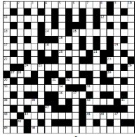
TCS Crossword

Try these:

• A confluence of researchers that generates fizz? (4)
• Fundamental fight (6,4)
• If the marking is right, it will fire! (8)

Find more clues like these and the grid in the TCS Crossword that was handed out to attendees during a coffee-break.

Algorithmic Contest (for students)

There was an algorithmic-contest as part of the conference (hosted on Algo Muse). Here is a take-away puzzle:

Contiguous t-sum problem. Given an array A[1..n] and a number t as input, find out if there exists a sub-array whose sum is t. For example, if the input is the array shown below and t=8, the answer is YES since A contains the sub-array A[2..4] whose sum is t. Prove an Ω(n log n) lower bound for the above problem on a comparison model.